
Implement Tabular Q-Learning and Inspect the Q-Table
The Q-learning update looks like a ritual until you print the table before and after training and watch the numbers crawl toward the goal.

Key topics
The Q-learning update looks like a ritual until you print the table before and after training and watch the numbers crawl toward the goal.
That is the whole point of this build. You already have a tiny environment that you verified: states, actions, rewards, and terminal behavior that behave the way you expect. You have also read the conceptual explanation of Q-learning, so you know the update rule and why the target takes a max over next actions. Now you turn that rule into code, run it, and inspect the result.
By the end you will have three things: a script that trains end to end, a Q-table you can actually read, and a baseline comparison that either passes or points at a bug.
What You Are Building and What Counts as Success
The deliverable is one sentence long: a tabular Q-learning agent trained on your verified toy environment, plus a printed Q-table and a comparison against random actions.
Before you start, confirm your prerequisites:
- The verified environment from the earlier build article, already smoke-tested for transitions, rewards, and terminal behavior.
- Basic Python and NumPy.
- A way to run a script and read its output.
Define success before you write a line of code, so you cannot quietly move the goalposts:
- The script runs end to end without error.
- The Q-table changes from its zero initialization.
- Greedy rollouts after training reach the goal more often than a random-action baseline, and among successful episodes, in fewer steps.
You will write three moving parts: the Q-table, the epsilon-greedy action selector, and the update step. Everything else is a loop that glues them together.
This works because your environment is small and discrete. Every state-action pair gets its own cell, so a table is the right data structure. When states multiply beyond what you can enumerate, the same update logic needs a function approximator instead. That is a later problem.
Connect the Code to Your Environment
The snippets below assume a small interface. Your verified environment may expose these under different names, so adapt the adapter once, at the top, and leave the rest of the script untouched.
# Adapter: map your verified environment onto the interface used below.
# Required attributes and methods:
#   env.n_states      -> int, number of discrete states
#   env.n_actions     -> int, number of discrete actions
#   env.grid_shape    -> tuple, for reshaping the policy for display
#   env.reset()       -> int, starting state
#   env.step(action)  -> (next_state, reward, done)

import numpy as np

n_states = env.n_states
n_actions = env.n_actions
If your environment returns a tuple from reset() or a five-tuple from step(), unwrap it here once. Do not scatter that adaptation through the training loop; every later bug becomes harder to see.
Set Up the Q-Table and Hyperparameters
Start with the smallest runnable piece: the table itself.
q_table = np.zeros((n_states, n_actions))
print(q_table.shape)  # (n_states, n_actions)
Starting at zero is a neutral, common choice. It implies something important: early on, every action in a state looks equally good, so argmax is ambiguous. Break ties randomly, or the agent will lock onto whichever action happens to sit at index zero.
Now the three knobs:
| Hyperparameter | Plain meaning | Starting value |
|---|---|---|
| Learning rate (alpha) | How far each update moves the estimate | 0.1 |
| Discount (gamma) | How much future reward counts | 0.95 |
| Epsilon | How often the agent explores | 0.2 |
These are starting points for a tiny deterministic environment, not sacred constants. Print the all-zero table now. That is your "before" image, and you will compare against it later.
Note: With all zeros,
np.argmaxreturns the first index on a tie. That is a silent action bias, not a decision. Always break ties randomly.
Knowledge check
Check your understanding
Answer this question before you continue.
Write the Epsilon-Greedy Action Selector
This function generates the experience the agent learns from.
def choose_action(state, q_table, epsilon, rng):
    if rng.random() < epsilon:
        return int(rng.integers(q_table.shape[1]))  # explore
    values = q_table[state]
    best = np.flatnonzero(values == values.max())
    return int(rng.choice(best))  # exploit, ties broken randomly
This is the behavior policy — the rule that picks actions during training. It is not the same as the greedy policy the table is learning toward. You saw that distinction conceptually; here it lives in code, in the if branch.
Keep epsilon fixed for the first run. That isolates the learning mechanism. Decaying epsilon is a later experiment, not a requirement.
The observable check: set epsilon near 1 and actions look random. Set it near 0 and the agent repeats its current best guess.
Knowledge check
Check your understanding
Answer this question before you continue.
Implement the Q-Learning Update
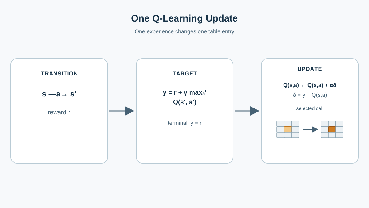
One function, five inputs.
def update(q_table, state, action, reward, next_state, done, alpha, gamma):
    if done:
        target = reward
    else:
        target = reward + gamma * np.max(q_table[next_state])
    td_error = target - q_table[state, action]
    q_table[state, action] += alpha * td_error
    return td_error
Break the target into its parts: the reward you just received, plus the discounted best value of where you landed. The gap between that target and your current estimate is the TD error. The update nudges the estimate toward the target by a fraction of that gap.
The terminal case is where beginners lose hours. When the episode ends, there is no next state to bootstrap from, so the target is just the reward. Skip that check and the goal reward never propagates cleanly backward.
Watch one transition move:
old value: 0.00
reward: 1.0, gamma: 0.95, max next: 0.0
target: 1.00
td error: 1.00
new value: 0.10
That is the same max-over-next-actions target from the conceptual article, now applied to one row of a real table.
Knowledge check
Check your understanding
Answer this question before you continue.
Run the Training Loop and Watch the Table Change
Assemble the pieces.
rng = np.random.default_rng(0)
alpha, gamma, epsilon = 0.1, 0.95, 0.2

for episode in range(500):
    state = env.reset()
    done = False
    while not done:
        action = choose_action(state, q_table, epsilon, rng)
        next_state, reward, done = env.step(action)
        update(q_table, state, action, reward, next_state, done, alpha, gamma)
        state = next_state
Print the table after the first episode, after a handful, and at the end. The change tells a story. Early updates are noisy and local — only the states the agent happened to touch move at all. Later, value propagates backward from the goal as the agent revisits states along the path.
The signature of learning is visible: the action leading toward the goal accumulates the highest value in each state along the route. The table is the agent's entire memory here. No neural network, no hidden state — just numbers you can read.
Read the Learned Policy From the Table
Turn the table into a policy.
policy = np.argmax(q_table, axis=1)
print(policy.reshape(env.grid_shape))
Walk through two or three states and ask why the chosen action is reasonable given the reward structure. In a state one step from the goal, the action that steps onto the goal should carry the highest value. In a state two steps away, the value should be smaller but still point the right way.
Now the caution. Distinguish states the agent visited often from states it barely visited. Poorly visited states may hold unreliable values — the table reflects the experience collected, not an oracle. This is the inspection payoff: the matrix stops being a matrix and becomes a map of decisions.
Compare Against a Random Baseline
Proof, not trust. Define the baseline plainly: an agent that picks uniformly random actions each step. The evaluation must report both goal-success rate and steps among successful episodes, because a policy that fails fast can otherwise look efficient.
def evaluate(policy_fn, episodes=100):
    successes = 0
    success_steps = []
    for _ in range(episodes):
        state = env.reset()
        done = False
        count = 0
        while not done:
            action = policy_fn(state)
            state, _, done = env.step(action)
            count += 1
        if done and state == env.goal_state:
            successes += 1
            success_steps.append(count)
    rate = successes / episodes
    mean_steps = np.mean(success_steps) if success_steps else float("nan")
    return rate, mean_steps

greedy = lambda s: int(np.argmax(q_table[s]))
random_policy = lambda s: int(rng.integers(n_actions))

print("greedy:", evaluate(greedy))
print("random:", evaluate(random_policy))
If your environment does not expose goal_state, track success inside the loop by checking the terminal reward instead. The point is that the metric must distinguish reaching the goal from merely stopping.
Run evaluation with exploration off, so you measure the learned policy rather than the exploration noise. Keep the comparison honest: same environment, same starting conditions, same number of evaluation episodes.
The trained greedy policy should reach the goal more often than random, and among successful episodes, in fewer steps. If it does not, that is a signal, not a failure of the exercise. Go to the next section.
Knowledge check
Check your understanding
Answer this question before you continue.
Debug the Three Failures Beginners Hit
Flat table. Values never move. Check that update is actually called inside the loop and that alpha is not zero. A single misplaced indent can leave the table frozen at zeros.
Agent never reaches the goal. Epsilon may be too low early, gamma too small, or terminal handling wrong so the goal reward never propagates. Print the target on the step that lands on the goal. If it is not just the reward, your done flag is not reaching the update.
Greedy policy looks random. Ties are not broken randomly, or you trained for too few episodes for values to separate. Print the max-minus-second-max gap per state. If it is near zero everywhere, the values have not separated yet.
One more: confirm your environment's state identifiers map directly to table rows. An off-by-one here produces a table that learns something — just not about the states you think.
Each failure is evidence about what the system is doing. Read it that way.
One Experiment Worth Running Next
Change one thing at a time. Decay epsilon over episodes and watch whether the learned policy stabilizes faster or the agent gets stuck exploiting a mediocre path:
epsilon = max(0.05, 1.0 - episode / 300)
Or hold epsilon fixed and vary the learning rate. Compare how quickly the table converges and whether it overshoots. Record the before-and-after table or the baseline metric so the change is measured, not assumed.
A surprising result is the useful part. If faster decay produces a worse policy, you just learned something concrete about the exploration-learning loop: the agent stopped gathering the information it needed before it had enough.
Where This Leaves You
Here is your decision rule. If your greedy policy beats random on both success rate and successful-episode length, you have a working tabular Q-learning agent and a readable Q-table. That is the checkpoint. If it does not, the failure is almost always terminal handling, exploration settings, or too few episodes — check them in that order.
The table works because your state space is small enough to enumerate. The moment states multiply past what you can list, the same update logic needs a function approximator instead of a lookup table. That is the next practical direction, and it is the reason the tabular version is worth building by hand first: you now know exactly what the approximator is replacing.
Knowledge check
Final check
Finish the article by checking the ideas you just learned.
References
Build a stronger RL mental model
Use structured resources to connect equations, algorithms, and observable agent behavior.


