
Evaluate a Tabular RL Agent Across Repeated Runs
A single episode is one sample. A single seed is one opinion. If you want to know whether your tabular agent learned anything, stop reading one number and…

Key topics
A single episode is one sample. A single seed is one opinion. If you want to know whether your tabular agent learned anything, stop reading one number and start reading a distribution.
You already have a working Q-learning agent and a verified toy environment. You watched the Q-table fill in, and you confirmed that greedy behavior beats a random baseline. That was the right first check. It was also the easiest one.
Now the harder question shows up: is the change I just made actually better, or did I get a lucky seed? That question does not have a single-episode answer. It has a distribution answer, and building the habit of reading that distribution is the real skill in this exercise.
Why One Episode Proves Nothing
A return is the total reward collected in one episode. It is a single draw from a distribution shaped by three things: where the episode started, what the agent explored, and what the environment did in response. Change any of those and the return moves.
Two kinds of variation hide in that sentence, and it helps to name them separately.
Between-run variation comes from the training seed. A seed is the number that initializes the random number generator, so two runs with different seeds explore in different orders, visit different states early, and end up with slightly different Q-tables. A run is one independent training session with its own seed.
Within-run variation comes from episode-to-episode noise. Even inside a single run, the agent's greedy policy can land in a bad starting state or hit a short episode by chance. That is why a learning curve wobbles.
The failure mode is predictable. You run the agent once, see a high return, and report it. Or you run it ten times, keep the best one, and call that performance. Both are the same mistake wearing different clothes: you are reporting the maximum of a noisy sample and calling it the mean.
Common mistake: Reporting the best run, or the last run, as "the result." Neither is a measurement. They are anecdotes with decimal points.
The prerequisite evaluation material already covered repeated episodes, seeds, and learning curves as concepts. Here we turn that into a runnable procedure: freeze the agent, run it many times, summarize the spread, then change exactly one knob and compare against the baseline.
Knowledge check
Check your understanding
Answer this question before you continue.
Set Up the Experiment Harness
The harness is the reusable asset. Write it once and every later experiment becomes a one-line change.
Assumptions: you have the tiny tabular environment and the tabular Q-learning agent from the earlier tutorials. No new dependencies are needed beyond what those already use.
The structure has three parts, and the separation matters:
- Train with exploration on, for a fixed budget.
- Evaluate with a greedy policy and no learning updates.
- Return per-episode evaluation returns, not just a mean, so variability stays visible.
import random
import statistics

def run_experiment(seed, n_train_episodes=500, n_eval_episodes=100):
    random.seed(seed)
    agent = QLearningAgent(env, alpha=0.1, gamma=0.99,
                           epsilon=1.0, epsilon_decay=0.995)

    # Train: exploration on, fixed budget.
    for _ in range(n_train_episodes):
        agent.train_episode(env)

    # Evaluate: greedy, no updates.
    eval_returns = [agent.evaluate_episode(env)
                    for _ in range(n_eval_episodes)]
    return eval_returns
Two design choices deserve a sentence each.
Fixed training budget. Every run gets the same number of training episodes. If you let one configuration train longer, you are comparing effort, not algorithms. The budget is the controlled variable.
Greedy evaluation. During evaluation, the agent picks the best-known action and does not update its Q-table. You want to measure the policy it learned, not the policy it is still exploring. Mixing exploration into evaluation adds noise you did not ask for.
The function returns a list of per-episode returns. Keep it that way. If you collapse to a mean inside the harness, you throw away the variability before you get a chance to look at it.
Expected observable output: a list of 100 floats per run, plus a printed summary line like seed=0 mean=8.42 std=2.10 min=3 max=13.
Knowledge check
Check your understanding
Answer this question before you continue.
Run It Many Times and Summarize the Spread
Now run the harness across a fixed list of seeds and summarize.
SEEDS = [0, 1, 2, 3, 4, 5, 6, 7, 8, 9]

run_means = []
for seed in SEEDS:
    returns = run_experiment(seed)
    run_means.append(statistics.mean(returns))
    print(f"seed={seed} mean={statistics.mean(returns):.2f} "
          f"std={statistics.stdev(returns):.2f} "
          f"min={min(returns)} max={max(returns)}")

print(f"\nacross runs: mean={statistics.mean(run_means):.2f} "
      f"std={statistics.stdev(run_means):.2f} "
      f"min={min(run_means):.2f} max={max(run_means):.2f}")
Report three numbers, not one. The mean tells you the center. The standard deviation tells you how consistent the agent is. The min and max tell you the worst and best cases, which is often what you actually care about.
A mean of 8.4 with a standard deviation of 0.3 describes a reliable agent. A mean of 8.4 with a standard deviation of 3.5 describes an agent that is occasionally brilliant and frequently mediocre. Those are different agents, and the mean alone cannot tell them apart.
For visualization, a strip plot or box plot of per-run means is enough. Plot the individual points, not just the box. Seeing ten dots spread across a range is more honest than a single bar.
Note: Use a fixed seed list. If you let the seeds change between experiments, you cannot tell whether a difference came from your change or from the seeds. Reproducibility is not a formality here; it is the thing that makes the comparison fair.
Sanity check before you trust anything: run the same configuration twice with the same seed list and confirm you get identical numbers back. If you do not, something in your harness is using randomness you did not seed.
Common mistake: Silently reusing the same seed for every run. You will get a tight, beautiful spread that means nothing, because you ran the same experiment ten times.
Knowledge check
Check your understanding
Answer this question before you continue.
Change One Thing: Baseline vs Variant
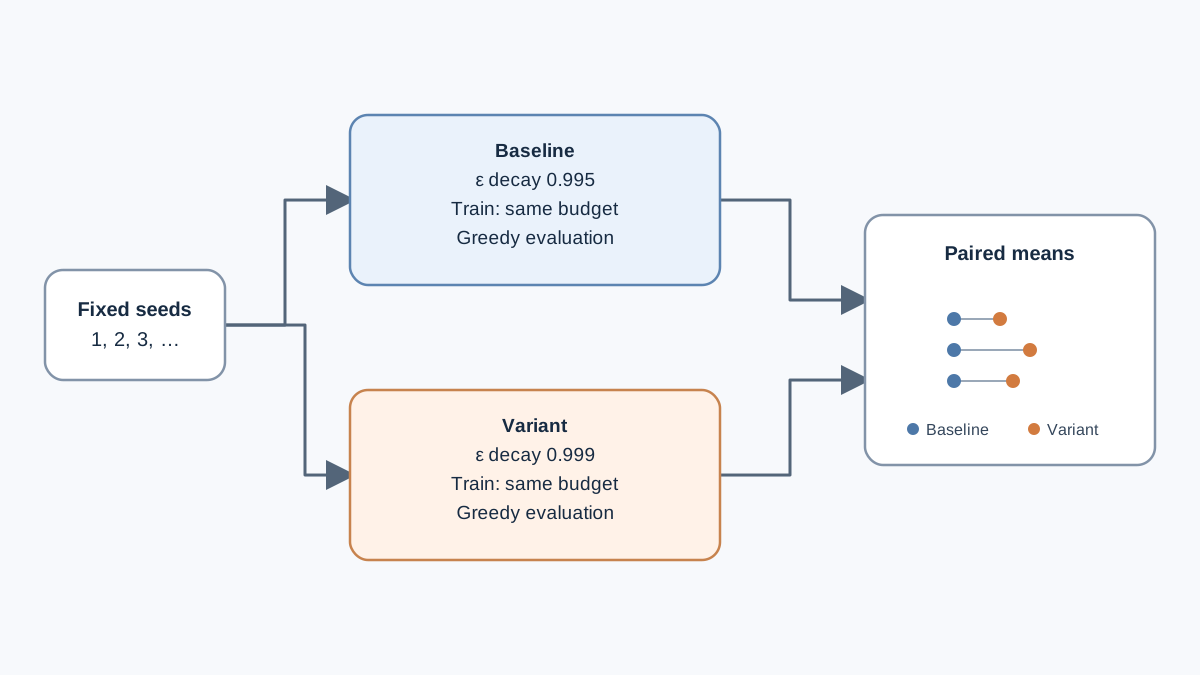
Here is where the harness pays off. Pick one knob, change only it, and write down what you expect before you run.
Say your hypothesis is that a slower epsilon decay will help, because the agent will explore longer before committing. Change epsilon_decay from 0.995 to 0.999. Keep the environment, the seed list, the training budget, and the evaluation procedure frozen.
def run_variant(seed):
    random.seed(seed)
    agent = QLearningAgent(env, alpha=0.1, gamma=0.99,
                           epsilon=1.0, epsilon_decay=0.999)
    for _ in range(500):
        agent.train_episode(env)
    return [agent.evaluate_episode(env) for _ in range(100)]
Then compare paired runs. For each seed, look at the baseline mean and the variant mean side by side. Do not just compare the two overall averages.
| Seed | Baseline mean | Variant mean | Difference |
|---|---|---|---|
| 0 | 8.42 | 8.90 | +0.48 |
| 1 | 7.10 | 7.85 | +0.75 |
| 2 | 9.30 | 9.10 | -0.20 |
| 3 | 6.80 | 8.20 | +1.40 |
The paired view tells you something the overall means hide: the variant wins on most seeds but loses on one. That is a different story from "the variant is better."
The decision rule: if the variant's advantage is smaller than the run-to-run spread, you cannot yet claim an improvement. Run more seeds before you believe it. A higher mean with fully overlapping distributions is weak evidence, not a result.
One boundary worth stating plainly: this procedure tells you whether a change helped on this task with this budget. It does not generalize to other environments. A slower epsilon decay that helps here might hurt on a task with a longer horizon.
Knowledge check
Check your understanding
Answer this question before you continue.
Read the Results Without Fooling Yourself
The experiment can lie to you in specific, repeatable ways. Here are the ones I see most often.
Comparing best-of-N against a single baseline run. If you ran the variant ten times and the baseline once, you are comparing a maximum to a sample. Run both the same number of times.
Changing two knobs at once. If you change the learning rate and the exploration schedule together, you cannot attribute the result to either one. Change one thing.
Tuning on the evaluation seeds. If you try configurations until one looks good on your seed list, you have overfit to those seeds. Hold out a fresh set for the final check.
Stopping when the numbers look good. This is the quiet one. You run seeds until the variant pulls ahead, then stop. That is not evidence; that is a search for a flattering summary.
Watching only the final mean. An agent that wins early and degrades has a fine final mean and an unstable policy. Plot the learning curve per run. Instability that a mean hides is often the most important thing to see.
When results are ambiguous, the honest move is to say so and increase the number of seeds. Keep a short experiment log: the seed list, the budget, the one change, and the summary numbers. That log is what makes the next comparison possible.
Your Next Experiment
Two concrete follow-ups, both cheap.
Expand the seed list. Rerun the same comparison with twenty or thirty seeds and see whether the conclusion holds. If the variant's advantage shrinks as you add seeds, it was probably noise.
Vary only the exploration schedule. Hold the algorithm fixed and sweep epsilon decay across a few values. This isolates how much of the outcome is exploration-driven, which is a question worth answering before you touch anything else.
A null result is a real result. Knowing that a change did not help is the skill this exercise is actually teaching. The harness you built here is the same structure you will need when you move from tabular methods to function approximation, where variance is larger and evaluation discipline matters more. Build the habit now, while the numbers are small enough to check by hand.
Knowledge check
Final check
Finish the article by checking the ideas you just learned.
References
Build a stronger RL mental model
Use structured resources to connect equations, algorithms, and observable agent behavior.


