Compare SARSA and Q-Learning on a Risky Path

Two agents train on the same grid, with the same rewards, the same learning rate, and the same epsilon. One learns to hug the edge of a penalty band. The other drifts wide around it. Nothing in the update formula you memorized explains that gap — the difference lives in what each target assumes about the next action.

This is a controlled experiment to make that difference visible. You will build one small risky-path task, run both tabular updates through it with persistent exploration, evaluate both learned policies the same way, and compare routes and returns across several seeds. By the end you will have a reusable procedure, not just a claim.

What This Experiment Is Actually Testing

The claim under test is narrow: with exploration that never fully stops, the SARSA target and the Q-learning target can produce different learned routes and different episode outcomes on the same task.

The claim not under test is that SARSA is universally safer. That is a property of one task, one reward shape, and one exploration schedule. Change any of those and the ranking can move. Hold onto that boundary — it is the difference between understanding a mechanism and repeating a slogan.

A quick bridge to what you already know. SARSA bootstraps on the action the behavior policy actually selects next. Q-learning bootstraps on the greedy action, regardless of what the behavior policy would pick. That is the whole on-policy versus off-policy distinction in one sentence. We will not re-derive it here; we will watch it produce different behavior.

To keep the comparison honest, fix everything else:

• Same grid, same reward function
• Same learning rate alpha, same discount gamma, same epsilon
• Same episode budget
• Same set of random seeds for both algorithms

One deliberate design choice: keep epsilon constant during training. Decaying epsilon hides the target difference, because as exploration fades, both targets converge toward the same greedy behavior. Persistent exploration is the microscope here. If you turn it off, you have nothing to look at.

The Risky Path Task and Its Reward Shape

We need the smallest environment where the target difference is visible. A plain maze will not do it — without a costly region, both algorithms tend to converge to the same route and the experiment teaches nothing.

Picture a small grid. A start cell, a goal cell, and a band of high-penalty cells forming a short corridor that runs right next to the goal. Beside that corridor is a longer, safe detour. The risky route is shorter. The safe route is longer. The penalty on the risky cells is what makes the detour competitive.

S . . . . . . . . G
. . . . . . . . . .
. . X X X X X X . .
. . . . . . . . . .

S is start, G is goal, X marks the risky band. The greedy-looking route runs along the row above the band; the cautious route drops down and around.

The reward shape:

• A small negative step cost on every move, so longer routes cost more.
• A large negative penalty on risky cells.
• A terminal reward at the goal.

The ratio between the penalty and the step cost is what makes the safe detour worth taking. If the penalty is tiny, the short risky route wins outright. If it is enormous, both algorithms learn the same detour and you learn nothing. Tune it so the two routes are genuinely close in value — that is where the target difference shows up.

We keep state and action as plain integers so the Q-table stays inspectable. No frameworks, no neural networks, no replay buffers. Just a table you can print.

Build the Shared Environment and Q-Table

Assumptions: Python 3 and NumPy. Nothing else. No external services, no credentials.

import numpy as np

GRID_W, GRID_H = 10, 4
START = (0, 0)
GOAL = (9, 0)
RISKY = {(x, 1) for x in range(2, 8)}  # the penalty band

STEP_COST = -1.0
RISKY_PENALTY = -100.0
GOAL_REWARD = 0.0

ACTIONS = [(-1, 0), (1, 0), (0, -1), (0, 1)]  # left, right, up, down
N_ACTIONS = len(ACTIONS)

def to_state(cell):
    return cell[1] * GRID_W + cell[0]

def to_cell(state):
    return (state % GRID_W, state // GRID_W)

def step(state, action):
    x, y = to_cell(state)
    dx, dy = ACTIONS[action]
    nx, ny = min(max(x + dx, 0), GRID_W - 1), min(max(y + dy, 0), GRID_H - 1)
    nxt = to_state((nx, ny))
    if (nx, ny) in RISKY:
        return nxt, RISKY_PENALTY, False
    if (nx, ny) == GOAL:
        return nxt, GOAL_REWARD, True
    return nxt, STEP_COST, False

N_STATES = GRID_W * GRID_H
Q = np.zeros((N_STATES, N_ACTIONS))

Zero initialization is fine here, but know what it does: every action starts tied at zero, so argmax breaks ties by picking the lowest index. That is arbitrary, not meaningful. It matters later when you read route traces — a tie can send the agent in an unexpected direction for reasons that have nothing to do with the target.

One shared action selector, used by both algorithms:

def epsilon_greedy(Q, state, epsilon, rng):
    if rng.random() < epsilon:
        return rng.integers(N_ACTIONS)
    return int(np.argmax(Q[state]))

Because both algorithms call this same function, the only thing that differs between runs is the update target. That is the controlled variable.

Quick sanity check before training:

s = to_state((3, 0))
nxt, r, done = step(s, 3)  # move down into the risky band
print(nxt, r, done)        # expect a large negative reward

If that prints the penalty, your environment is wired correctly.

Two Update Targets, One Training Loop

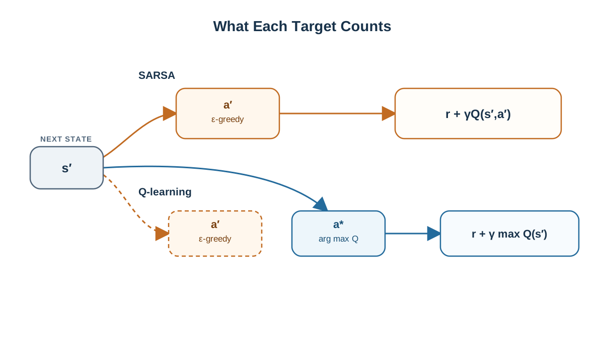
Here is the entire difference between the two algorithms, in two lines:

# SARSA: bootstrap on the action the behavior policy actually picks
target = r + GAMMA * Q[s_next, a_next] * (not done)

# Q-learning: bootstrap on the best estimated next action
target = r + GAMMA * np.max(Q[s_next]) * (not done)

That is it. Everything else — the environment, the selector, the table, the loop structure — is shared.

The structural consequence is worth noticing. SARSA needs a_next before it can update, so its loop carries the tuple (s, a, r, s', a'). Q-learning does not, because it never asks what the behavior policy would do next.

Now the mechanism, in plain terms:

• The max target is optimistic under exploration. It credits a future action the exploring agent may never take. If the agent is about to wander randomly into a penalty cell, Q-learning's target does not price that in.
• The SARSA target is pessimistic under exploration. It prices in the chance that the next action is a random one. The value it learns reflects the policy the agent is actually running, exploration and all.

Neither is "correct." They answer different questions. Q-learning asks: what is the best policy available from here? SARSA asks: what is the value of the policy I am actually executing?

def train(algorithm, episodes, alpha, gamma, epsilon, seed):
    rng = np.random.default_rng(seed)
    Q = np.zeros((N_STATES, N_ACTIONS))
    for _ in range(episodes):
        s = to_state(START)
        a = epsilon_greedy(Q, s, epsilon, rng)
        done = False
        while not done:
            s_next, r, done = step(s, a)
            if algorithm == "sarsa":
                a_next = epsilon_greedy(Q, s_next, epsilon, rng)
                target = r + gamma * Q[s_next, a_next] * (not done)
                Q[s, a] += alpha * (target - Q[s, a])
                s, a = s_next, a_next
            else:
                target = r + gamma * np.max(Q[s_next]) * (not done)
                Q[s, a] += alpha * (target - Q[s, a])
                s = s_next
                a = epsilon_greedy(Q, s, epsilon, rng)
    return Q

Keep the update as a single readable expression. Resist the urge to add function approximation or replay here — those change the question you are asking.

Separate Training From Evaluation

This is the step beginners skip, and it is the step that makes the comparison mean anything.

Train with epsilon held constant. Evaluate with epsilon set to zero and no learning updates. Training returns are contaminated by exploration noise. A lower training return does not mean a worse policy — it often means a noisier one. If you judge behavior from training episodes, you are measuring the exploration schedule, not the learned policy.

def evaluate(Q, max_steps=200):
    s = to_state(START)
    route, total = [s], 0.0
    for _ in range(max_steps):
        a = int(np.argmax(Q[s]))
        s, r, done = step(s, a)
        route.append(s)
        total += r
        if done:
            break
    return route, total

Report two things per algorithm: the greedy route taken during evaluation, and the distribution of evaluation returns across repeated runs. Run multiple seeds and report the spread. One seed is an anecdote, not a result.

seeds = range(10)
for algo in ("sarsa", "q_learning"):
    returns = []
    for seed in seeds:
        Q = train(algo, episodes=2000, alpha=0.5, gamma=0.99,
                  epsilon=0.1, seed=seed)
        _, total = evaluate(Q)
        returns.append(total)
    print(algo, np.mean(returns), np.std(returns))

Expected output is a route trace per algorithm plus a small table of mean and spread. If your spread is enormous, you probably need more episodes before the values settle.

Reading the Results: Routes, Returns, and What They Do Not Prove

The typical pattern on this kind of task: the Q-learning route tracks closer to the risky band, the SARSA route drifts wider, and SARSA's evaluation returns are often less variable across seeds. The mechanism is the one we named earlier — the max target ignores the cost of exploratory mistakes, so the learned values understate the risk the agent actually faces while exploring.

Aspect	SARSA	Q-learning
Target	r + γ Q(s', a')	r + γ max Q(s')
Policy learned	On-policy (behavior)	Off-policy (greedy)
Behavior during training	Cautious near risk	Aggressive near risk
Route tendency	Wider detour	Closer to the band
Return variability	Often lower	Often higher

Common mistake: Reading this table as a safety ranking. It is not one. It is a snapshot of one task under one exploration schedule.

What this does not prove: no universal safety guarantee. Change the penalty size, the epsilon value, or the episode horizon and the ranking can shift. The mechanism is durable; the verdict is not.

Failure modes to expect:

• Neither algorithm reaches the goal with too few episodes. Increase the budget.
• Ties in argmax produce arbitrary routes. Break ties deliberately if you care about reproducibility.
• Penalty too large and both agents learn the identical detour — the experiment stops teaching anything.

Change One Thing and Re-Run

The experiment becomes a method when you start varying one input at a time.

Modification: raise epsilon and re-run both algorithms with the same seeds.

Write down your prediction before running. Mine: SARSA's route should move further from the risky band, and the gap between the two routes should widen. The reason is mechanical — higher epsilon means more random next actions, and SARSA's target prices those in more heavily.

A second optional modification: shrink the risky-cell penalty and watch whether the two routes converge. If the penalty is small enough, the max target and the on-policy target agree on the same route, and the difference disappears.

Why this drill matters: it teaches that the target difference is a mechanism, not a fixed verdict, and that the exploration schedule is a first-class experimental variable.

Debugging signals if nothing changes when epsilon changes:

• Check that evaluation is actually greedy — a stray epsilon in evaluate will mask everything.
• Check that the update is using the intended target. A copy-paste slip between the two branches is easy to miss.
• Check that training episodes are enough for values to converge before you compare.

Where to Go Next

Close with a decision rule, not a summary. When you care about the policy your exploring agent will actually execute, read the SARSA target. When you care about the best policy available and can tolerate the cost of exploration, read the Q-learning target.

The next real constraint appears when the state space grows too large for a table. That is where function approximation enters, and with it the overestimation problem that the max target quietly invites. The mechanism you just watched in a 40-cell grid does not disappear when you replace the table with a network — it gets harder to see, and more expensive to ignore.