Experiment With TD(λ) and Eligibility Traces in a Small RL Task

Watch a one-step TD learner on a short corridor. The reward sits at the far end, and the value of the first state crawls upward for hundreds of episodes. Nothing is broken. The update only ever nudges the state right before the reward, so credit has to walk backward one step per episode while the agent keeps re-walking the same hallway.

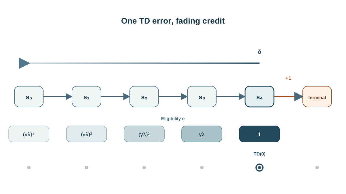
The fix is not a bigger learning rate. It is letting a single TD error reach further back in time. That is what eligibility traces do, and the cheapest way to believe it is to run the same task three ways and change only one number.

What You Are Actually Comparing

Three learners, one task:

• One-step TD (λ = 0): update V(S_t) toward R + γV(S_{t+1}).
• Tabular TD(λ) with an accumulating trace: spread that same TD error backward over recently visited states.
• Complete-return baseline: accumulate the discounted return from each visited state and update toward it at episode end.

The single independent variable is λ. Learning rate, discount, task, episode count, and random seed stay fixed. If you change two things, you learn nothing.

The trace version is not a different algorithm so much as a wider brush. One-step TD paints one state per step. The trace version paints every state whose trace is still warm, with the brush fading as you go back in time. If the mechanism itself feels shaky, the prerequisite pieces on eligibility traces and Monte Carlo versus TD cover the derivation; here we only need the update rule.

Declare your assumptions before you write code: tabular state space, episodic task, deterministic transitions, no function approximation. Every one of those is load-bearing.

State the success criterion up front, so the experiment can fail honestly: after N episodes, the value of the start state should approach the true expected return. We will measure episodes-to-threshold for each method.

The Small Task and Why It Exposes Credit Assignment

Use a corridor of five non-terminal states plus a terminal state. The agent starts at state 0, moves right with probability 1, and receives reward 1 on entering the terminal state. Every other transition pays 0.

The true value of state i under a discount γ is γ^(n-i), where n is the number of steps to the terminal. With γ = 0.9 and five steps from state 0, V(0) = 0.9^5 ≈ 0.590. Print that number. It is the ground truth that turns this from vibes into an experiment.

This task is the right microscope for one reason: the reward is delayed, so the only way early states learn is through credit propagating backward. It is also deliberately too simple to show the variance problems that make Monte Carlo painful in long or noisy episodes. Do not over-generalize from a five-state hallway.

Implementing the Three Learners

One environment, one episode loop, three update functions. Resist writing three separate scripts — the shared skeleton is what makes the comparison honest.

import numpy as np

N_STATES = 6          # 0..4 non-terminal, 5 terminal
TERMINAL = 5
GAMMA = 0.9
ALPHA = 0.1
EPISODES = 200

def run_episode(V, lam, traces=None):
    s = 0
    if traces is not None:
        traces[:] = 0.0
    while s != TERMINAL:
        s_next = s + 1
        r = 1.0 if s_next == TERMINAL else 0.0
        delta = r + GAMMA * V[s_next] - V[s]
        if traces is None:
            V[s] += ALPHA * delta
        else:
            traces[s] += 1.0
            V += ALPHA * delta * traces
            traces *= GAMMA * lam
        s = s_next
    return V

The one-step path is the traces is None branch. The trace path increments the current state's trace by 1, applies the TD error to every state weighted by its trace, then decays the whole trace vector by γλ.

The complete-return baseline needs a different shape, because it cannot update until the episode ends:

def run_episode_mc(V):
    s = 0
    visited = []
    while s != TERMINAL:
        visited.append(s)
        s += 1
    G = 0.0
    for s in reversed(visited):
        G = 1.0 + GAMMA * G if s == visited[-1] else GAMMA * G
        V[s] += ALPHA * (G - V[s])
    return V

Two implementation details matter more than they look.

Common mistake: Forgetting to reset traces to zero at the start of every episode. The trace vector is per-episode state. If it leaks across episodes, values drift upward without bound and you will blame the algorithm for a bug in your loop.

Note: The trace update applies to all states, not just the current one. If you only update V[s], you have written one-step TD with extra bookkeeping.

Print the value table every 25 episodes. For all three methods, V[0] should rise monotonically toward 0.590. The interesting result is how many episodes each one needs.

Running the Comparison

The payoff of this experiment is a single number per method: how many episodes until V[0] crosses a threshold. Define that threshold explicitly, then run all three learners and report the result.

TRUE_V0 = GAMMA ** 5
THRESHOLD = 0.95 * TRUE_V0   # within 5% of ground truth

def episodes_to_threshold(lam, seed=0):
    np.random.seed(seed)
    V = np.zeros(N_STATES)
    traces = np.zeros(N_STATES) if lam is not None else None
    for ep in range(1, EPISODES + 1):
        if lam is None:
            run_episode_mc(V)
        else:
            run_episode(V, lam, traces)
        if V[0] >= THRESHOLD:
            return ep
    return EPISODES  # never converged within budget

for lam in [0.0, 0.5, 0.9, 0.99]:
    print(f"lambda={lam}: {episodes_to_threshold(lam)} episodes")

print(f"complete returns: {episodes_to_threshold(None)} episodes")

Run it. On this deterministic corridor you will see one-step TD take the longest, intermediate λ values arrive sooner, and the complete-return baseline land somewhere in between — its updates are exact but only happen once per episode, so it learns in a handful of episodes rather than crawling.

That last result surprises people. The complete-return baseline is not slow here. It is slow when episodes are long and returns are noisy, not when the corridor is five steps and the reward is guaranteed.

Warning: One seed proves nothing. Rerun with several seeds before concluding which λ wins. A single lucky run is a story, not a result.

Sweeping Lambda: What Changes and What Does Not

Sweep λ over [0, 0.5, 0.9, 0.99], hold everything else fixed, and record episodes-to-threshold for each. The complete-return baseline is a separate row, not a λ value — it uses a different update rule, not a different decay setting.

Method	Credit propagation	Bias	Variance
λ = 0.0 (one-step TD)	One state per step	High	Low
λ = 0.5	Several states per step	Medium	Medium
λ = 0.9	Broad backward reach	Lower	Higher
λ = 0.99	Nearly full-episode reach	Very low	High
Complete returns	Full episode, once	None	Highest

The expected pattern on this corridor: performance improves as λ moves away from 0, then flattens or degrades as λ approaches 1 and the estimator inherits more of the complete-return variance.

The practical reading is that λ is not a knob you tune to a universal best value. It trades bias for variance, and the right setting depends on episode length, reward sparsity, and how noisy the returns are.

Reach for traces when episodes are long, reward is delayed, and the state space is small enough to keep a trace vector. Skip them when episodes are short enough that one-step TD already converges quickly, or when the extra bookkeeping costs more than it buys.

Note: The clean equivalence between the online trace update and the forward view holds exactly only for offline updates. The online version is an approximation. That is a known boundary, not a bug in your code.

Failure Modes and Debugging Signals

Treat a broken run as evidence, not a dead end.

• Values exploding or drifting upward: traces were not reset between episodes, or the decay was applied before the increment.
• TD(λ) matching one-step TD exactly: λ is effectively zero, or the trace vector is being reallocated each step instead of carried forward.
• TD(λ) matching the complete-return baseline exactly: λ is at or near 1, or the trace is never decayed.
• Divergence at high learning rate: the trace method diverges faster than one-step TD, because each step now touches many states at once. The effective step size grew.

Tip: With λ = 0, your trace implementation should reproduce the one-step TD numbers exactly. If it does not, the bug is in the trace code, not the algorithm.

Where This Leaves You

λ is a bias-variance dial, not a magic constant. The way to choose it is to measure episodes-to-threshold across a sweep on your own task rather than trusting a default.

The next practical step is to replace the tabular value table with a small function approximator, or move the same trace logic onto state-action values. The trace mechanism you just implemented is the same one that appears inside modern value estimators — the corridor is small, but the pattern scales.