Deriving N-Step TD Returns: Bootstrapping Between One-Step TD and Monte Carlo

One-step TD updates fast but bets on a guess. Monte Carlo waits for the whole episode but trusts only what happened. The n-step return asks a sharper question: what if you could look exactly n rewards ahead, then guess the rest?

That question has a clean answer, and the answer is worth deriving rather than memorizing. Once you can build the n-step target from scratch, you stop treating it as a library constant and start treating it as a dial you can reason about.

This article is about prediction targets. We are not building a full control algorithm here. We are answering one question: given a trajectory and a value estimate, what number should the value estimate move toward?

Where the One-Step Target Runs Out of Road

You already know the one-step target. It is the immediate reward plus a discounted estimate of the next state's value:

$y_t^{(1)} = r_{t+1} + \gamma V(s_{t+1})$

That target has two weaknesses, and they pull in opposite directions.

First, delayed reward propagates slowly. If a reward arrives twenty steps after the decision that caused it, a one-step update only moves the value of the state right before the reward. The signal has to crawl backward one state per update. In a long episode with sparse reward, that crawl is the bottleneck.

Second, the target leans hard on $V(s_{t+1})$. If that estimate is wrong, the update is wrong. You are training a prediction against another prediction, and early in learning the second prediction is mostly noise.

Monte Carlo fixes both problems by waiting. It uses the full observed return, so no bootstrap error enters the target and delayed reward propagates in one shot. The cost is that you cannot update anything until the episode ends, and the full return carries all the variance of every random reward and transition along the way.

The n-step return sits between these two. You collect n real rewards, then bootstrap from the value estimate at the horizon. Small n behaves like TD. Large n behaves like Monte Carlo. The rest of this article derives that target, computes one by hand, and handles the case where the episode ends before you reach the horizon.

Notation Before the Formula

The algebra is short, but only if every symbol is already pinned down.

Symbol	Meaning
$t$	Current time step
$s_t$	State at time $t$
$a_t$	Action taken at time $t$
$r_{t+1}$	Reward received after taking $a_t$
$\gamma$	Discount factor, $0 \le \gamma < 1$ for continuing tasks
$V(s)$	Current estimate of the value of state $s$
$n$	Number of real rewards to collect before bootstrapping
$T$	Terminal time step of the episode

Two distinctions matter. A reward is something you observed. A value estimate is something you predicted. The n-step target mixes them, and keeping the two roles separate is what makes the derivation readable.

We assume a fixed policy is being evaluated, so the actions along the trajectory come from that policy. We also assume rewards are bounded. In a finite episodic task, that is enough to keep the return finite even when $\gamma = 1$. In a continuing task, the return is only guaranteed finite when $\gamma < 1$, so the rest of this article treats $\gamma < 1$ as the default and notes where the episodic case relaxes it.

Building the n-Step Return Step by Step

Start from the true return. From state $s_t$, the return is the discounted sum of everything that follows:

$G_t = r_{t+1} + \gamma r_{t+2} + \gamma^2 r_{t+3} + \cdots$

This is the Monte Carlo target. It is unbiased if you actually observe the whole trajectory, but you cannot compute it until the episode ends.

Now truncate it after n rewards:

$G_t = \underbrace{r_{t+1} + \gamma r_{t+2} + \cdots + \gamma^{n-1} r_{t+n}}_{\text{observed}} + \underbrace{\gamma^n r_{t+n+1} + \gamma^{n+1} r_{t+n+2} + \cdots}_{\text{tail}}$

The first block is real data. The tail is everything you have not seen yet.

Here is the move that defines the method. Factor $\gamma^n$ out of the tail:

$\text{tail} = \gamma^n \left( r_{t+n+1} + \gamma r_{t+n+2} + \cdots \right) = \gamma^n G_{t+n}$

The quantity inside the parentheses is exactly the return from state $s_{t+n}$ onward. You do not know it, but you have an estimate of its expected value: $V(s_{t+n})$. Replace the tail with that estimate:

$y_t^{(n)} = \sum_{k=0}^{n-1} \gamma^k r_{t+k+1} + \gamma^n V(s_{t+n})$

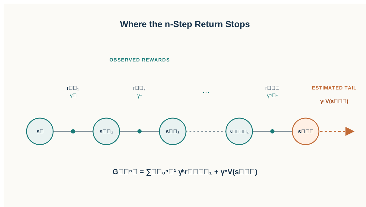
That is the n-step return. Read it as a sentence: collect n real rewards, discount each by its distance, then add a discounted guess about everything after the horizon.

Why the Bootstrap Carries $\gamma^n$

This is the detail people get wrong most often, so it is worth slowing down.

The value estimate $V(s_{t+n})$ stands in for the entire return starting at time $t+n$. But that return is measured from time $t+n$, not from time $t$. To express it in the units of the current target, you have to discount it back across the n steps you already skipped. Each skipped step contributes one factor of $\gamma$. After n steps, that is $\gamma^n$.

If you use $\gamma$ instead of $\gamma^n$, you are pretending the future estimate sits one step away when it actually sits n steps away. The target becomes too large, and the error grows with n.

The Two Boundary Cases

Check the formula at both ends.

Set $n = 1$. The sum runs over $k = 0$ only, giving $r_{t+1}$, and the bootstrap term is $\gamma^1 V(s_{t+1})$. That is the familiar one-step TD target. Nothing new.

Now suppose the episode ends at step $T$ and $n$ reaches that boundary. There is no state $s_{t+n}$ to evaluate, so the bootstrap term disappears and the target collapses to the plain discounted sum of the remaining rewards. That is Monte Carlo for the rest of the episode.

Between those two cases, n is a dial. Turn it down and you trust your estimate more. Turn it up and you trust your data more.

Picture a timeline. Filled segments for the n observed rewards, each one discounted a little more than the last. Then a dashed segment at the horizon, labeled $\gamma^n V(s_{t+n})$, standing in for everything past the edge of what you can see.

A Worked Example You Can Check by Hand

Numbers make this concrete. Take a deterministic chain of states with $\gamma = 0.9$ and a fixed policy. Suppose you start at $s_t$ and observe this sequence:

Step	Reward
$r_{t+1}$	2
$r_{t+2}$	4
$r_{t+3}$	6

Suppose the current value estimates are $V(s_{t+1}) = 10$, $V(s_{t+2}) = 8$, and $V(s_{t+3}) = 5$.

One-step target:

$y_t^{(1)} = 2 + 0.9 \cdot 10 = 2 + 9 = 11$

Two-step target:

$y_t^{(2)} = 2 + 0.9 \cdot 4 + 0.9^2 \cdot 8 = 2 + 3.6 + 6.48 = 12.08$

Three-step target:

$y_t^{(3)} = 2 + 0.9 \cdot 4 + 0.9^2 \cdot 6 + 0.9^3 \cdot 5 = 2 + 3.6 + 4.86 + 3.645 = 14.105$

Look at what changed across the three targets. The one-step target is dominated by the estimate of 10. The three-step target is dominated by observed rewards, and the bootstrap contributes only 3.645. As n grows, the target depends more on what happened and less on what you guessed.

You can verify the same arithmetic in code. This is a check on the hand calculation, not a replacement for it:

gamma = 0.9
rewards = [2, 4, 6]
values = [10, 8, 5]  # V(s_{t+1}), V(s_{t+2}), V(s_{t+3})

for n in (1, 2, 3):
    observed = sum(gamma**k * rewards[k] for k in range(n))
    bootstrap = gamma**n * values[n - 1]
    print(f"n={n}: {observed + bootstrap:.3f}")

Run it. You should see 11.000, 12.080, and 14.105. If your hand arithmetic matches the output, the formula is yours.

When the Episode Ends Before n Steps

This is the single most common place where n-step targets go silently wrong, and it splits into two cases that look similar and behave differently.

True Terminal State

Suppose the episode terminates at step $T$, and $T < t + n$. You cannot bootstrap from $s_{t+n}$ because that state never happens. The correct target is the plain discounted sum of the rewards you actually collected:

$y_t^{(n)} = \sum_{k=0}^{T-t-1} \gamma^k r_{t+k+1}$

No bootstrap term. None.

Why does bootstrapping past termination break things? Because there is no future value to estimate. If you plug in $V(s_{t+n})$ anyway, you inject phantom reward into the target. Values near episode ends get inflated, and the inflation spreads backward through every update that touches those states.

Time-Limit Cutoff

Now the case that trips people up. Suppose the environment cuts the episode at step $T$ because a step budget ran out, not because the task is over. The future still has value. You just cannot see it from inside this episode.

The target is the same shape as the ordinary n-step return, but with the horizon moved to the cutoff. Sum the rewards you observed up to $T$, then bootstrap from the value of the final observed state, discounted by the number of steps you actually took:

$y_t^{(n)} = \sum_{k=0}^{T-t-1} \gamma^k r_{t+k+1} + \gamma^{T-t} V(s_T)$

The exponent is $T - t$, not $n$, because you only skipped $T - t$ steps before reaching the state you are bootstrapping from. This is the truncated-return-plus-bootstrap target, and it is what you want whenever the episode ended for bookkeeping reasons rather than task reasons.

Common mistake: Treating a time-limit cutoff the same as a true terminal state. If the environment ends the episode because a step budget ran out, the future may still have value. If the episode ends because the task is genuinely over, it does not. These two cases need different targets.

The practical rule is to track the episode boundary explicitly and branch on it. When you form the target, ask two questions. Did the horizon step exist? If yes, bootstrap from $s_{t+n}$ with $\gamma^n$. If no, did the episode end because the task is over or because a limit was hit? Terminal means sum and stop. Time limit means sum and bootstrap from the last observed state with $\gamma^{T-t}$.

This branching has a cost. You cannot form the n-step target until you have buffered n rewards, which means your update pipeline needs a queue of pending transitions. That bookkeeping is the real price of multi-step targets, and it is worth knowing before you reach for a large n.

Choosing n: Bias, Variance, and the Cost of Waiting

There is no universally correct n. There is only a tradeoff you can measure.

n	Bias	Variance	Update delay
Small	High (trusts the bootstrap)	Low	Short
Large	Low (trusts observed rewards)	High	Long

Small n inherits the bias of your value estimate. If the estimate is systematically off, the target is systematically off, and the update chases a wrong number. But small n also averages over fewer random rewards, so the target is stable.

Large n inherits the variance of the trajectory. Every random reward and every stochastic transition along the way enters the target. The bias shrinks because you are relying less on the estimate, but the noise grows. You also wait longer before any update is possible, and you buffer more experience.

The bias reduction only holds while the horizon stays inside the episode. Once n exceeds the remaining episode length, every target collapses to the same Monte Carlo sum, and turning the dial further does nothing. That is why the useful range of n is bounded by your typical episode length, not by how patient you feel.

My rule for a new task: start near the middle, measure, and adjust. Compare learning curves for a few values of n on the same environment. If updates look noisy and unstable, reduce n. If learning is slow and delayed rewards seem to take forever to propagate, increase n. The right value depends on your reward density, your episode length, and how good your value estimate is early on.

Note: The same interpolation idea generalizes into weighted mixtures of many n-step returns, where shorter and longer horizons are blended with decaying weights. That is a separate topic, but it is the natural next step from here.

Common Mistakes and How to Catch Them

Four errors account for most broken n-step targets.

Off-by-one in reward indexing. The first reward is $r_{t+1}$, not $r_t$. Rewards are received after actions, so the index is always one ahead of the state. If your targets are consistently shifted, check this first.

Using $\gamma$ instead of $\gamma^n$ on the bootstrap. The estimate covers everything after n steps, so it must be discounted by n steps. This error inflates targets, and the inflation grows with n.

Bootstrapping through a terminal state. Covered above, but it deserves repetition because it is invisible. The target looks reasonable. The values are just quietly wrong near episode ends.

Forgetting the behavior policy. The intermediate actions along the trajectory must come from the policy actually being followed. If you are evaluating one policy but collecting data from another, the target is measuring the wrong thing.

Here is the detection habit I use: hand-check one target against a brute-force full-episode return on a short deterministic episode. If the episode is short enough that you can compute the true return by hand, you can compare it to your n-step target with n set to the episode length. They should match exactly. When they do not, the bug is almost always one of the four above.

What This Unlocks Next

The core idea fits in one sentence: observe n real rewards, then guess the rest.

From here, the natural direction is eligibility traces, which blend many n-step returns into a single update without buffering n rewards. That is the mechanism that removes the bookkeeping cost you paid here.

For now, run the experiment. Implement the n-step target for a fixed policy on a small gridworld. Collect one trajectory. Compute the target for n = 1, n = 4, and n equal to the full episode length on that same trajectory. Then add a step-limit cutoff and compute the truncated-return-plus-bootstrap target for the same trajectory. Compare all four numbers. Watch how the target shifts from estimate-heavy to data-heavy as n grows, and how the time-limit case keeps a bootstrap where the terminal case drops it.

Then pick your n by measuring bias and variance on your own task. Not by copying a default. The dial is yours to turn, and now you know what each setting actually does.