Forward and Backward Views of Eligibility Traces: Deriving TD(λ)

You read one chapter that builds TD(λ) from a weighted mixture of n-step returns. You read another that updates a decaying trace and broadcasts the TD error backward. Both chapters call the result TD(λ). If you cannot tell whether those are the same algorithm or two close cousins, you are not missing a step—the equivalence is real, but it rests on assumptions that textbooks often leave implicit. This article derives the connection and names exactly when it holds.

We will keep the setting small on purpose: a fixed policy, a value function $V$, and a single trajectory of experience. That is enough to see the mechanism clearly. Once the algebra is on the table, the assumptions become visible instead of mysterious.

Two Descriptions of One Algorithm

The forward view asks: what target should we have used for the state we visited? It answers by looking ahead from that state, mixing returns of many lengths into one number. The backward view asks: given the error we just observed, which past states deserve credit? It answers by keeping a fading record and applying the error in proportion to that record.

One view is for understanding what is computed. The other is for building a mechanism that runs online. Before comparing them, fix the notation.

Symbol	Meaning
$\gamma$	discount factor, $0 \le \gamma \le 1$
$\lambda$	trace-decay / mixing parameter, $0 \le \lambda \le 1$
$\delta_t$	one-step TD error at time $t$
$e_t(s)$	eligibility trace for state $s$ at time $t$
$G_t^{(n)}$	n-step return from time $t$
$G_t^{\lambda}$	λ-return from time $t$
$\alpha$	learning rate

The equivalence claim, stated precisely: for a complete episode with off-line updates, the total change applied to each state's value by the forward view equals the total change applied by the backward view. Off-line means you accumulate all updates and apply them after the episode ends, rather than mutating $V$ mid-episode. Everything below either supports that claim or marks where it stops being true.

The Forward View: Mixing n-Step Returns

Start with the building block. The n-step return looks $n$ rewards ahead, then bootstraps with the current estimate:

$G_t^{(n)} = R_{t+1} + \gamma R_{t+2} + \cdots + \gamma^{n-1} R_{t+n} + \gamma^n V(S_{t+n})$

The λ-return is a geometric mixture of these, weighted so that shorter returns get more weight and longer returns fade:

$G_t^{\lambda} = (1 - \lambda) \sum_{n=1}^{\infty} \lambda^{n-1} G_t^{(n)}$

The weights $(1-\lambda)\lambda^{n-1}$ sum to 1, so this is a genuine average, not a scaled sum. Check the endpoints:

• At $\lambda = 0$, only the $n=1$ term survives: $G_t^{\lambda} = G_t^{(1)} = R_{t+1} + \gamma V(S_{t+1})$, the one-step TD target.
• At $\lambda = 1$, the mixture collapses onto the full return $G_t$, the Monte Carlo target.

So $\lambda$ is a dial between bootstrapping and waiting for the whole episode. The forward-view update for a visited state is simply $V(S_t) \leftarrow V(S_t) + \alpha\big(G_t^{\lambda} - V(S_t)\big)$.

The cost is structural. To compute $G_t^{\lambda}$ you need rewards that have not happened yet. The forward view is naturally an off-line or delayed method: you look forward, then update.

The Terminal Tail in an Episodic Task

The infinite mixture above is clean, but a real episode ends. Once $t + n$ passes the terminal step $T$, there is no $S_{t+n}$ to bootstrap from, so the convention is that every n-step return beyond termination equals the full return $G_t$:

$G_t^{(n)} = G_t \quad \text{for all } n \ge T - t$

Substituting that into the mixture, the tail collapses into a single residual weight on the full return:

$G_t^{\lambda} = (1 - \lambda) \sum_{n=1}^{T-t-1} \lambda^{n-1} G_t^{(n)} + \lambda^{T-t-1} G_t$

The weights still sum to 1. That residual term is not a technicality—it is exactly the $\lambda^2$ weight the worked example below relies on, and it is the reason $\lambda = 1$ recovers Monte Carlo even on a finite episode.

The Backward View: Traces as a Fading Record

The backward view flips the direction. Instead of looking forward from a state, it keeps a short-term memory of which states were recently visited. The accumulating trace recursion is:

$e_t(s) = \gamma \lambda \, e_{t-1}(s) + \mathbb{1}(S_t = s)$

Read it as two operations per step: decay every trace by $\gamma\lambda$, then add 1 at the state just visited. The update then applies the current TD error to every state in proportion to its trace:

$V(s) \leftarrow V(s) + \alpha \, \delta_t \, e_t(s) \quad \text{for all } s$

Why do $\gamma$ and $\lambda$ appear together? Both shrink influence with temporal distance. The discount $\gamma$ says a reward two steps away matters less than one step away; the trace decay $\lambda$ says a state two steps back is less eligible than one step back. Multiplying them means a single factor $\gamma\lambda$ controls how fast credit fades.

The payoff is timing. The backward view updates online, using only what has already happened. No waiting for the episode to end.

Deriving the Equivalence

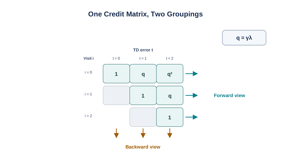
Now the algebra. The trick is to stop grouping by return and start grouping by TD error.

Write the forward-view update for a single state $s$ as a sum over every time it was visited. Under off-line updating, $V$ is frozen for the whole episode, so each visit contributes its own λ-return error:

$\Delta V(s) = \sum_{t=0}^{T-1} \alpha \, \mathbb{1}(S_t = s) \big(G_t^{\lambda} - V(S_t)\big)$

The next move is the one textbooks skip. A λ-return is not just a mixture of returns—it is also a weighted sum of TD errors. To see that, expand the n-step return as a telescoping series of one-step TD errors. Each $G_t^{(n)}$ can be written as $V(S_t)$ plus a chain of discounted TD errors:

$G_t^{(n)} - V(S_t) = \sum_{k=t}^{t+n-1} \gamma^{k-t} \delta_k$

This holds because the intermediate $V$ terms cancel: each $\gamma V(S_{k+1})$ from one step is subtracted by the $\gamma V(S_{k+1})$ inside the next $\delta_{k+1}$. Substituting this into the λ-return mixture and swapping the order of summation—summing over $k$ instead of over $n$—gives:

$G_t^{\lambda} - V(S_t) = \sum_{k=t}^{T-1} (\gamma\lambda)^{k-t} \delta_k$

The geometric mixture over $n$ has become a geometric sum over future TD errors, with the same decay factor $\gamma\lambda$. Now plug this back into the forward-view total change:

$\Delta V(s) = \sum_{t=0}^{T-1} \alpha \, \mathbb{1}(S_t = s) \sum_{k=t}^{T-1} (\gamma\lambda)^{k-t} \delta_k$

Exchange the two sums—group by $\delta_k$ instead of by visit time $t$:

$\Delta V(s) = \sum_{k=0}^{T-1} \alpha \, \delta_k \sum_{t=0}^{k} (\gamma\lambda)^{k-t} \, \mathbb{1}(S_t = s)$

Look at the inner sum. It accumulates 1 each time state $s$ was visited at or before step $k$, decaying by $\gamma\lambda$ for every step since. That is exactly the accumulating trace $e_k(s)$. So:

$\Delta V(s) = \sum_{k=0}^{T-1} \alpha \, \delta_k \, e_k(s)$

The coefficient multiplying each $\delta_k$ is the trace value at that time. The forward-view total and the backward-view total are the same number. That is the derivation—not a coincidence, but a regrouping of the same sum.

Note: With on-line updating, the two views differ slightly, because the forward view uses the original $V$ values to compute every target while the backward view mutates $V$ as it goes. The gap shrinks as $\alpha \to 0$, which is why the equivalence is stated for off-line updates.

A Worked Trace on a Tiny Episode

Make it concrete. Take a three-step episode with $\gamma = 1$, $\lambda = 0.5$, $\alpha = 0.1$, and a single terminal reward of 1 at the end. Suppose all values start at 0, and the trajectory visits states $A \to B \to C \to$ terminal.

The TD errors are $\delta_0 = 0$, $\delta_1 = 0$, $\delta_2 = 1$ (the reward arrives at the last step). Only the final error is nonzero, so the forward view assigns the entire update through the λ-return of each state. For state $A$ at $t=0$, the terminal tail gives weight $\lambda^{T-t-1} = 0.5^2 = 0.25$ on the full return, which is why $A$'s update is smaller than $C$'s.

Compute the traces step by step with $\gamma\lambda = 0.5$:

Step	Visited	$e(A)$	$e(B)$	$e(C)$
0	A	1.0	0	0
1	B	0.5	1.0	0
2	C	0.25	0.5	1.0

At step 2, $\delta_2 = 1$, so the backward update is $\Delta V(s) = 0.1 \times 1 \times e_2(s)$: $A$ gets $0.025$, $B$ gets $0.05$, $C$ gets $0.1$. The forward view, computing each λ-return and summing the resulting changes, produces the same three numbers under off-line updating. Run it on-line and you get a small mismatch, because $C$'s update changes the target used for $B$ and $A$.

Common mistake: Forgetting to reset traces at the terminal step. If $e(A)$ survives into the next episode, the first TD error of the new episode credits a state from the old one. The update looks plausible and is silently wrong.

Accumulating vs Replacing Traces

The recursion above is the accumulating variant. A state visited twice in one episode gets 1 added twice, so its trace can exceed 1. The replacing trace sets the visited state's trace to 1 instead of adding:

$e_t(s) = \begin{cases} 1 & \text{if } s = S_t \\ \gamma\lambda \, e_{t-1}(s) & \text{otherwise} \end{cases}$

Both fit the same backward update; only the trace recursion changes. The difference matters when states repeat within an episode. Large accumulated traces can destabilize tabular learning or slow convergence, so replacing traces are often the safer default when revisits are common.

Here is the boundary that trips people up. The derivation above proves exact forward-backward equivalence for accumulating traces. Replacing traces change the eligibility coefficients whenever a state is revisited, so the same λ-return regrouping does not carry over automatically. Replacing traces are a useful variant with a different forward view, not a relabeling of the same identity. If you want the exact equivalence, use accumulating traces; if you use replacing traces, verify the behavior empirically rather than assuming the identity holds.

When the Equivalence Holds, and When It Breaks

The clean identity depends on a short list of assumptions. Name them, and the boundaries become obvious.

• Off-line updates over a complete episode. This is the exact case. On-line updates are close but not identical.
• Accumulating traces. The proof above is specific to the accumulating recursion. Replacing traces are a separate variant.
• Tabular or linear value function. With a linear parameterization, the same regrouping holds in weight space. With nonlinear approximation, the backward view becomes a practical approximation, not an identity—stale gradients from earlier parameters can misassign credit.
• Episodic termination handled explicitly. Terminal states need their traces zeroed, and the $\lambda = 1$ case in continuing tasks needs separate treatment because there is no final return to fall back on.
• On-policy. Off-policy settings introduce importance-sampling corrections that change the trace itself, so the clean equivalence no longer applies directly.

Warning: If you are using a neural network critic and assuming exact forward-backward equivalence, you are assuming something the math does not give you. Treat the backward view as the implementable approximation it is.

What This Buys You

Use the forward view to reason about what a method is optimizing. Use the backward view to implement it online. When the two disagree in your code, the disagreement is a diagnostic, not a bug to hide.

Pick $\lambda$ as a bias-variance dial, not a magic constant. Low $\lambda$ leans on bootstrapping—lower variance, more bias. High $\lambda$ leans on real returns—less bias, more variance. The best value depends on your task, and you should expect to tune it.

My rule: implement both views on the same small episodic task and compare the weight trajectories before trusting either. If they match off-line and diverge on-line, you have confirmed the derivation and found the boundary in one experiment. If they never match, check your trace reset at the episode boundary first—that is the failure that hides longest.