Eligibility Traces in Reinforcement Learning: A Bridge Across Time

One-step TD updates are beautifully local: take a step, observe the reward and next state, correct the value of the state you just left. Then you hit the problem every RL beginner eventually hits. The reward that matters arrives ten steps after the decision that caused it, and your one-step update cannot reach back that far.

Eligibility traces close that gap. They keep a fading record of what you recently did, so when a TD error finally fires, it reaches backward and updates every recent decision at once—weighted by how fresh each one is.

The Gap One-Step TD Leaves Open

Think about what a one-step TD update does in causal terms. At time step t, you were in state Sₜ, took an action, and landed in Sₜ₊₁ with reward Rₜ₊₁. The update corrects the value of Sₜ based on the difference between what you predicted and what actually happened one step later. That is a local correction: it adjusts the state immediately before the reward or next state appeared.

Now consider a delayed reward. You make a decision, wander through several intermediate states, and only then receive a meaningful reward. The decision that caused it sits many steps behind you. One-step TD has no direct route to reach it. Credit must propagate backward one visit at a time, through repeated encounters with the same states, like a rumor traveling slowly down a hallway.

This is the temporal credit assignment problem you already know: the late reward belongs to earlier actions, but the learning rule has no way to connect them directly. Monte Carlo solves this by waiting until the episode ends and using the full return. One-step TD solves it by being patient—eventually, after enough visits, value information diffuses backward. But "eventually" can mean a lot of episodes.

The question this article answers: how do you update many past decisions at once, without waiting for the episode to end the way Monte Carlo does?

The Mental Model: A Fading Record of What You Just Did

An eligibility trace is a short-term memory. Every time you visit a state or take an action, you flag it as recently involved. Then, each step, every flag fades by a decay factor. Recent events stay bright. Older ones dim toward zero.

Picture a trail of footprints in fresh snow. The prints closest to you are sharp and deep. Walk a few more steps, and the earlier prints blur. Walk far enough, and they disappear entirely. The trace works the same way: it marks where you have been, with the most recent marks carrying the most weight.

The analogy is exact in one important sense: the trace encodes both recency and frequency. A state visited often stays eligible even if its last visit was several steps ago, because each visit adds fresh ink. A state visited once and never again fades quickly. This dual encoding matters more than most explanations admit—it is why traces handle repeated states gracefully rather than treating each visit as an isolated event.

How One Error Reaches Backward

Here is the elegant trick at the heart of trace-based learning. Instead of looking forward n steps to compute a multi-step return, you propagate the current TD error backward through the trace.

When a TD error fires, you multiply it by each state's trace value. Recent states get a large correction. Distant states get a small one. States you never visited get nothing at all.

The update shape is simple:

value change = learning rate × TD error × trace value

That single multiplication does a surprising amount of work. One error signal updates many states at once, in a single pass, without storing the whole episode. You do not need to remember what happened ten steps ago in detail—the trace already compressed that history into a single number per state.

This is called the backward view of TD(λ), and it has a conceptual twin: the forward view, which looks ahead and computes n-step returns. The forward view asks, "If I look n steps into the future, what return should I expect?" The backward view asks the mirror question: "If an error happens now, which past states deserve credit?"

Under the right conditions, these two views produce identical updates. The backward view is not a separate idea—it is a practical shortcut that reproduces what the forward view would compute, without the bookkeeping. That equivalence is why traces matter: they give you the power of multi-step learning with the efficiency of a one-step update.

A Tiny Walkthrough: Watching One Error Spread

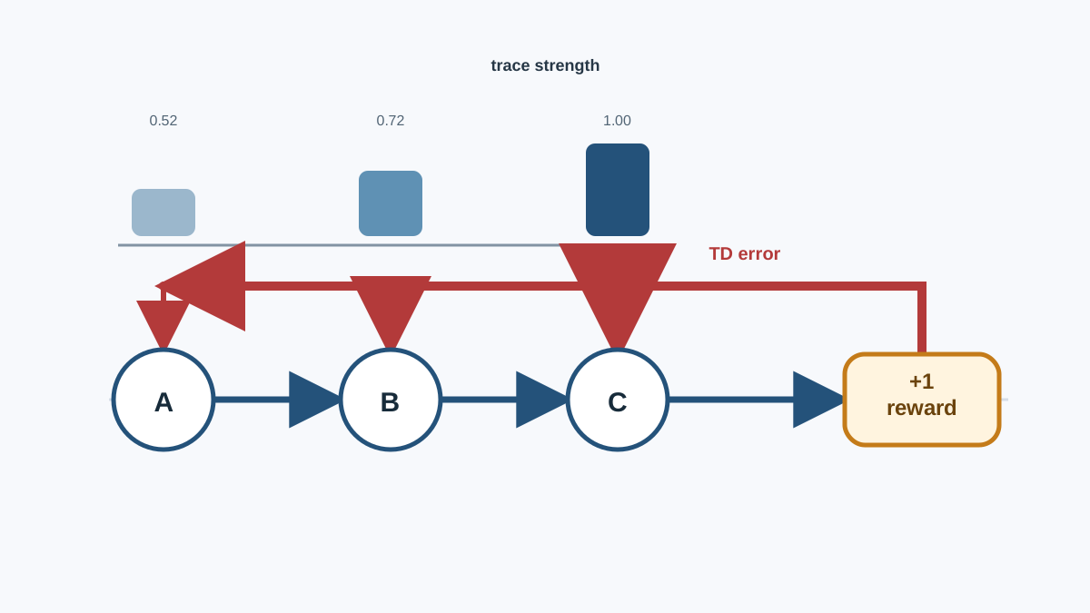
Let us make the mechanism concrete. Imagine a three-state corridor: A → B → C. The agent receives a reward of +1 only when it reaches C. No other step produces a reward. Suppose the agent has just completed this trajectory, and its current value estimates are all zero.

Choose γ = 0.9 and λ = 0.8. The trace for each state decays by γ × λ = 0.72 per step, then adds 1 when the state is visited. After visiting A, B, and C in sequence, the trace values are roughly:

• State A: 0.72 × 0.72 ≈ 0.52
• State B: 0.72
• State C: 1.0

Now the agent reaches C and observes the +1 reward. The TD error is:

δ = reward + γ × V(next state) − V(current state)

With no next state after C, the error simplifies to roughly δ = 1.0. One error fires, and every state on the corridor updates at once:

• A changes by α × 1.0 × 0.52
• B changes by α × 1.0 × 0.72
• C changes by α × 1.0 × 1.0

That is the bridge in action. One-step TD would have updated only C. The trace lets the same error reach A and B in a single pass, with the correction shrinking as the trace fades.

Note: The trace distributes credit according to recency and visitation. It does not prove which action caused the reward—it assigns more blame or praise to decisions that were recent when the error arrived.

Lambda as a Dial Between TD and Monte Carlo

The decay rate of the trace is controlled by a parameter called λ (lambda). It is the dial that decides how far back your memory reaches.

Set λ = 0, and the trace forgets everything instantly. Only the most recent state gets updated. You have recreated one-step TD.

As λ approaches 1, the trace fades more slowly, and the method leans toward longer-return, Monte Carlo-like learning. The exact endpoint depends on your formulation and how you handle episode termination, but the direction is consistent: higher λ means credit reaches further back.

Set λ somewhere in between, and you get an exponentially weighted blend of all possible n-step returns. Recent states get strong updates. Older ones get weaker ones. This middle ground often beats either extreme.

The reason comes down to the bias-variance tradeoff. Short traces are biased—they only see local information, so they systematically underestimate the consequences of distant decisions. But they are low-variance, because each update depends on only a few noisy steps. Long traces are less biased—they see more of the actual return—but they are noisier, because more random steps contribute to each update.

One warning before you tune: λ interacts with the discount factor γ. The combined decay rate is γ × λ. If your problem has a long horizon and a discount factor well below 1, you need a high λ to reach far enough back. A λ of 0.9 with a γ of 0.9 gives an effective decay of 0.81 per step—after ten steps, the trace has faded to roughly 12% of its original strength. Choose λ with your discount factor in mind, not in isolation.

Note: The λ parameter is where the name TD(λ) comes from. When you see TD(λ) in a paper or implementation, it means temporal-difference learning with an eligibility trace controlled by λ.

Accumulating vs Replacing Traces

When you read actual implementations, you will encounter two different rules for updating the trace itself. The distinction is a frequent source of confusion, so it is worth recognizing both.

An accumulating trace adds to the existing value each time you visit a state. Visit a state, and its trace goes up by 1. Visit it again, and it goes up by another 1. The trace accumulates evidence of repeated visits.

A replacing trace resets the trace to 1 each time you visit a state, instead of adding. The trace never grows beyond 1 for any single state, no matter how many times you visit it in a row.

Why does the distinction matter? Accumulating traces can over-weight states that are visited many times in succession. Imagine an agent stuck in a loop, visiting the same state twenty times in a row. An accumulating trace would give that state a trace value of 20 or more, letting one TD error produce an outsized update. A replacing trace caps the contribution at 1.

My rule for beginners: do not treat this as a free choice. Use the trace convention the algorithm you are implementing specifies, document which one you chose, and test repeated-state behavior deliberately. If you see strange oscillations in your value estimates, check which trace rule your implementation uses before changing anything else.

When Traces Earn Their Keep and When They Do Not

Eligibility traces shine when three conditions hold: rewards are delayed, episodes are long, and you want faster credit propagation without waiting for episode end. If your agent must navigate a maze for fifty steps before finding a reward, a trace lets every state in that path receive credit the moment the reward arrives—not after repeated visits spread the information backward.

Traces earn less keep when rewards are immediate, when the environment has a short horizon, or when you already use a method that handles multi-step credit another way. If your agent gets feedback every step, one-step TD is already doing the right thing. Adding traces adds complexity without adding much benefit.

An honest note on the modern landscape: many deep RL systems do not use classic tabular traces directly. They rely on n-step returns, Generalized Advantage Estimation (GAE), or replay buffers to handle multi-step credit. But the trace idea did not disappear—it got absorbed. GAE, in particular, is conceptually close to a trace mechanism for advantage estimation. Understanding traces gives you a clearer picture of what those modern methods are actually doing under the hood.

The boundary is worth stating plainly: traces are a clean, powerful idea in tabular settings, and they are one tool among several in deep RL—not a universal answer.

The Experiment That Makes It Click

The fastest way to internalize this idea is to run a tiny tabular experiment. Build a short corridor where the agent must choose left or right at the start, then walk several steps before receiving a reward that depends on that initial choice. The delayed reward is the whole point: the agent cannot see the consequence of its first decision until several steps later.

Train three agents with the same step size and random seed: one with λ = 0 (one-step TD), one with an intermediate λ around 0.5, and one with λ = 0.9. Track two things: how many episodes each agent needs before its value estimates stabilize, and the trace values themselves as the episode progresses.

What result would confirm the mechanism? The λ = 0 agent should learn eventually, but slowly, because credit must diffuse backward one visit at a time. The trace-based agents should propagate the reward backward immediately, producing visible corrections in the earlier states on the very episode the reward arrives. You do not need a dramatic winner—you need to see the difference in when the earlier states start changing.

If the trace-based agents do not learn faster, do not assume traces failed. Check your trace update rule, confirm the decay factor γ × λ is not too aggressive for your corridor length, and verify that the reward is genuinely delayed rather than leaking through your state representation. The experiment teaches the mechanism only when you can inspect the trace values and see where credit is flowing.

Keep the durable mental model: a trace is a fading record that lets one error reach back across time. Recent decisions get the strongest correction. Older ones get a fainter echo. And the λ dial decides exactly how far back that echo travels.

References

Research updated Sep 9, 2026