
Measure Q-Learning Overestimation With a Noisy-Value Experiment
You have read that Q-learning overestimates. You nodded. You moved on. But you have never seen the bias as a number, so it stays a rumor.

Key topics
You have read that Q-learning overestimates. You nodded. You moved on. But you have never seen the bias as a number, so it stays a rumor.
Here is the reframe that makes it click: the bias is not a bug in the update rule. It is what happens when you ask a noisy estimate to pick a winner. Maximization does not average noise. It selects the top of it.
Let's build a thirty-line experiment that turns that sentence into a measurement — and then corrects it.
Why the Max Picks the Loudest Estimate
Start with the mental model before any code.
Imagine five actions. All five are genuinely worth the same: true value 1.0. Your agent does not know that. It only has estimates, and every estimate is the true value plus some error:
estimate = true_value + noise
The noise is symmetric. Sometimes an action looks better than it is, sometimes worse. If you averaged the five estimates, the positive and negative errors would cancel and you would land near 1.0. Averaging is honest.
Maximization is not. When you take the maximum, you are not asking "what is the typical value?" You are asking "which action looks best right now?" And the action that looks best is usually the one whose noise happened to land high.
With equally valued actions, the true maximum is the same value for every action. So any positive deviation wins the selection. The expected maximum of noisy estimates is therefore greater than the maximum of the true values:
E[ max(estimates) ] > max( true values )
That gap is maximization bias. It is a property of the selection step, not of any single sample. This is the mechanism behind the Q-learning overestimation bias experiment we are about to run, and it is the same mechanism that shows up when a Q-learning target takes a max over noisy next-state values.
Note: The bias comes from the max operator, not from the noise being "wrong." Zero-mean noise is fine. Maximizing it is what tilts the result upward.
Knowledge check
Check your understanding
Answer this question before you continue.
The Smallest Experiment That Shows the Bias
You need Python and NumPy. No environment, no agent, no training loop. We are isolating one step: select a maximum from noisy estimates and compare it to the truth.
import numpy as np

rng = np.random.default_rng(0)

TRUE_VALUE = 1.0
N_ACTIONS = 10
NOISE_SCALE = 1.0
N_TRIALS = 20_000

gaps = []
for _ in range(N_TRIALS):
    estimates = TRUE_VALUE + rng.normal(0.0, NOISE_SCALE, size=N_ACTIONS)
    selected = estimates.max()
    gaps.append(selected - TRUE_VALUE)

print(f"true value:        {TRUE_VALUE:.3f}")
print(f"mean selected:     {TRUE_VALUE + np.mean(gaps):.3f}")
print(f"measured bias:     {np.mean(gaps):.3f}")
Run it. The mean selected value sits above 1.0, and the gap is the measured bias. With ten actions and a noise scale of one, that gap is roughly one unit — the max is picking estimates that are about a full standard deviation above the truth.
Read the code as three distinct quantities, because conflating them is where beginners get lost:
| Quantity | What it is | In the code |
|---|---|---|
| True value | The real worth of each action | TRUE_VALUE |
| Noisy estimate | What the agent sees | estimates |
| Selected maximum | What the max operator returns | estimates.max() |
The bias is the average distance between the third and the first. A single trial proves nothing — one run can land below the true value. The repeated-trial average is the success criterion.
Knowledge check
Check your understanding
Answer this question before you continue.
Reading the Output: What the Numbers Mean
Two knobs control the size of the bias, and both are testable.
Number of actions. More actions means more chances for some estimate to land high. The max of ten noisy draws beats the max of two.
Noise scale. Wider noise means a taller upper tail to grab. Shrink NOISE_SCALE toward zero and the bias shrinks with it. At exactly zero noise, the bias is zero — which is correct, not a broken experiment.
Try it. Change N_ACTIONS to 2, then to 50. Change NOISE_SCALE to 0.1, then to 3.0. Watch the printed bias move. You are now measuring the thing you used to take on faith.
Common mistake: Trusting a single trial. If you run the loop once and see a value below
1.0, you have not disproved the bias. You have observed one sample from a distribution whose mean is above1.0. IncreaseN_TRIALSbefore you trust any gap.
Knowledge check
Check your understanding
Answer this question before you continue.
Fixing It: Select With One Estimate, Evaluate With Another
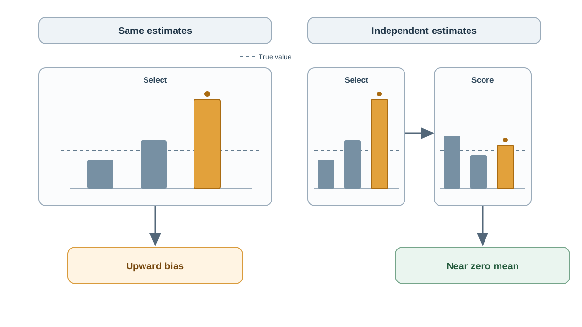
Here is the modification. Draw a second, independent set of noisy estimates. Use the first set only to choose the winning action. Use the second set only to score that action.
gaps_naive = []
gaps_double = []

for _ in range(N_TRIALS):
    selection = TRUE_VALUE + rng.normal(0.0, NOISE_SCALE, size=N_ACTIONS)
    evaluation = TRUE_VALUE + rng.normal(0.0, NOISE_SCALE, size=N_ACTIONS)

    # Naive: select and evaluate with the same noisy estimates
    best_naive = selection.max()
    gaps_naive.append(best_naive - TRUE_VALUE)

    # Independent: select with one set, evaluate with the other
    best_action = selection.argmax()
    gaps_double.append(evaluation[best_action] - TRUE_VALUE)

print(f"naive bias:        {np.mean(gaps_naive):.3f}")
print(f"independent bias:  {np.mean(gaps_double):.3f}")
The naive bias stays positive. The independent bias collapses toward zero.
Why? The winning action was chosen because its selection noise landed high. But the evaluation noise is uncorrelated with that selection noise, so the evaluation does not inherit the winner's upward error. The selection and the evaluation are decoupled.
This is the mechanism behind the Double Q-learning bias experiment. Double Q-learning maintains two value functions, uses one to pick the greedy action and the other to score it. We stay at the estimator level here — the full algorithm, with its two tables and update schedule, is a separate step.
Knowledge check
Check your understanding
Answer this question before you continue.
Failure Modes and Debugging Signals
When the fix looks useless, check these in order.
You reused the same noise. If selection and evaluation share the same array, the evaluation inherits the winner's error and the bias stays. The two estimates must be independent draws. This is the single most common way to break the experiment.
Too few trials. A noisy average can hide or exaggerate the gap. If your numbers jump around between runs, raise N_TRIALS before drawing conclusions.
Zero noise, zero bias. If you set NOISE_SCALE = 0.0 and see no bias, nothing is broken. No noise means no upper tail to grab.
The independent estimate can still wander. In this equal-value setup, the independent evaluation averages near zero bias, but any single run can land above or below the true value. That is sampling noise, not a flaw in the method. If you later test unequal action values, the independent estimator can undershoot the true maximum because selection may pick a suboptimal action — a separate case worth exploring once this one is solid.
Tip: When a result surprises you, isolate one variable. Change only
NOISE_SCALE, rerun, and compare. Debugging is applied reasoning — a surprising number is evidence about what the code actually did.
One More Experiment: Turn the Knobs
Now sweep. This is where the mental model becomes durable.
import numpy as np

rng = np.random.default_rng(1)
TRUE_VALUE = 1.0
N_TRIALS = 20_000

for n_actions in [2, 5, 10, 25, 50]:
    naive, double = [], []
    for _ in range(N_TRIALS):
        sel = TRUE_VALUE + rng.normal(0, 1.0, size=n_actions)
        evl = TRUE_VALUE + rng.normal(0, 1.0, size=n_actions)
        naive.append(sel.max() - TRUE_VALUE)
        double.append(evl[sel.argmax()] - TRUE_VALUE)
    print(f"actions={n_actions:>3}  naive={np.mean(naive):.3f}  independent={np.mean(double):.3f}")
Read the printed rows as the action count grows. The naive column climbs; the independent column stays near zero. Then swap the sweep to noise scale and watch the same pattern.
This is why real agents with many actions and imperfect value estimates drift optimistic. Every max over a noisy set is a small bet on the upper tail. Stack thousands of those bets across a training run and the optimism compounds.
Where This Leaves You
The decision rule is short: whenever a target takes a max over noisy estimates, expect optimism, and measure it before you trust it.
You now have a script that proves the bias, a modification that removes the selection-noise advantage in this toy setup, and two knobs that show you how it scales. The next practical step is to apply the same selection/evaluation split inside a real Q-learning update — pick the next action with one value function, score it with another, and use that score in the target. If you want the conceptual explanation of why the max fools the agent in the first place, that reasoning stands on its own and is worth reading separately before you wire the split into a full training loop.
Knowledge check
Final check
Finish the article by checking the ideas you just learned.
References
Build a stronger RL mental model
Use structured resources to connect equations, algorithms, and observable agent behavior.


