Compare Memoryless and Recurrent Policies in a Partially Observed Task

A memoryless agent can learn perfectly and still lose. It extracts every drop of signal from the observation it receives, then plateaus at a score a coin flip could match — not because training failed, but because the input never contained the answer.

This is a controlled experiment. One small task, two policies, identical training budget, one changed variable: whether the policy can see history. By the end you will have a runnable comparison, a visible performance gap, and a diagnostic habit for telling "memory would fix this" apart from "the observation design is broken."

If partial observability and recurrent policies are still fuzzy, the short version is enough to proceed: an observation that does not identify the hidden state makes the task non-Markovian over observations, so the optimal action can depend on history the agent cannot currently see. A memoryless policy is a function of the current observation alone. A history-dependent policy is a function of the current observation plus some summary of what came before. That is the entire variable we are testing.

Designing a Task Where History Actually Matters

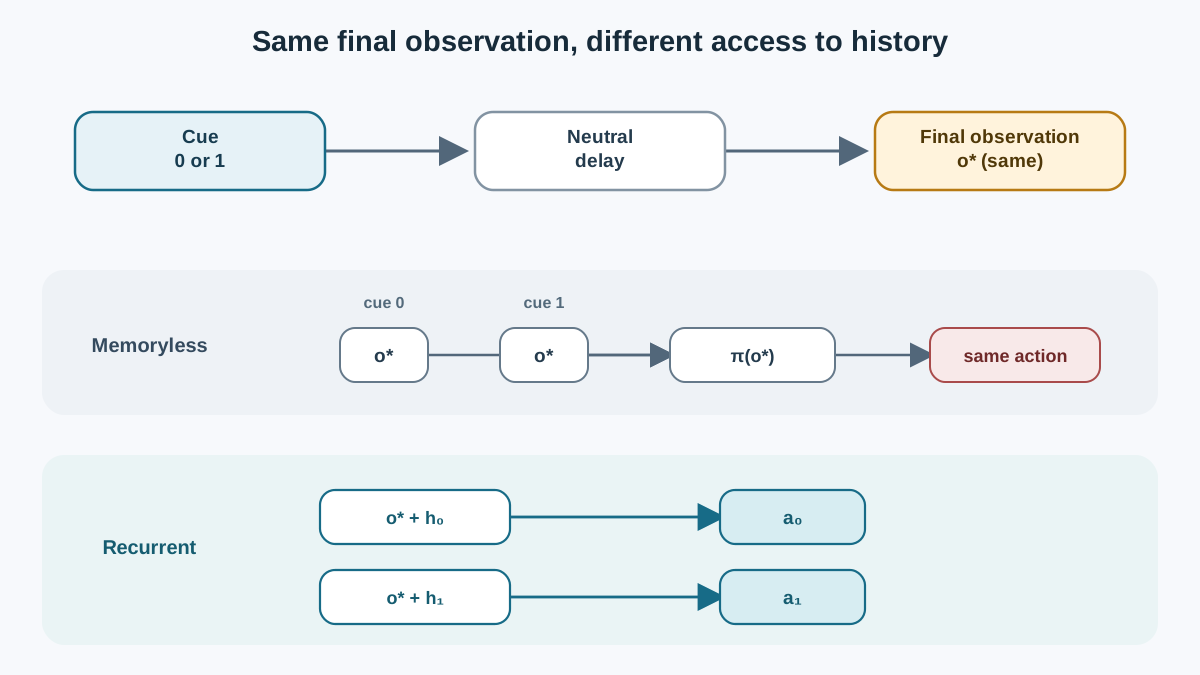
We need a task small enough to reason about by hand, where the current observation is deliberately insufficient and the required memory is short and interpretable.

Use a cue-then-act structure:

1. At step 0, the environment reveals a hidden context — call it a cue bit, either 0 or 1.
2. Steps 1 through delay emit a neutral observation. Nothing informative happens.
3. At the final step, the agent must choose action 0 or action 1. It gets reward +1 only if the action matches the cue bit from step 0.

The observation at decision time is identical in both cases. The reward is sparse but deterministic. A human reading the episode description knows exactly what to do: remember the cue, act on it. The agent sees a blank wall.

Why this is a fair test:

• The hidden variable is decision-relevant. The cue bit changes which action is correct.
• The observation is lossy by construction. The cue is visible once and then gone.
• The memory horizon is short. A recurrent state or a small history window can plausibly hold one bit across a handful of steps.

Now add the control. Build a fully observed version of the same task where the cue bit is included in every observation. Same reward structure, same delay, same action space. In that version, a memoryless policy should be sufficient — the current observation already contains the answer. If the memoryless policy still fails there, the problem is task difficulty, not observability. The control is what proves the gap comes from the missing information.

Note: Keep the state space tiny. Two cue values, a fixed delay, two actions. You want to be able to enumerate the correct policy in your head before you run anything.

Building the Environment and the Memoryless Baseline

Dependencies are minimal: Python, NumPy, and PyTorch for the policy network. No external services, no credentials, no GPU required.

The environment is a fixed-length episode. The observation vector has two slots: a cue slot and a step counter. In the partially observed version, the cue slot is zeroed after step 0. In the control version, it stays populated.

import numpy as np
import torch
import torch.nn as nn

class CueTask:
    def __init__(self, delay=4, fully_observed=False):
        self.delay = delay
        self.fully_observed = fully_observed
        self.obs_dim = 2
        self.n_actions = 2

    def reset(self):
        self.cue = np.random.randint(2)
        self.t = 0
        return self._obs()

    def _obs(self):
        cue_slot = self.cue if (self.fully_observed or self.t == 0) else 0
        return np.array([cue_slot, self.t / self.delay], dtype=np.float32)

    def step(self, action):
        done = self.t == self.delay
        reward = 1.0 if (done and action == self.cue) else 0.0
        self.t += 1
        return self._obs(), reward, done

The memoryless policy maps the current observation to action logits — deliberately no history, no recurrence:

class MemorylessPolicy(nn.Module):
    def __init__(self, obs_dim, n_actions):
        super().__init__()
        self.net = nn.Sequential(
            nn.Linear(obs_dim, 32),
            nn.ReLU(),
            nn.Linear(32, n_actions),
        )

    def forward(self, obs):
        return self.net(obs)

Now the rollout and training loop. This is the piece the earlier draft left implicit: rollout must actually construct episodes, sample actions, and return the log-probabilities and rewards the update needs.

def rollout(policy, env, recurrent=False):
    obs = env.reset()
    h = None
    logps, rewards = [], []
    done = False
    while not done:
        obs_t = torch.tensor(obs).unsqueeze(0)
        if recurrent:
            logits, h = policy(obs_t, h)
        else:
            logits = policy(obs_t)
        dist = torch.distributions.Categorical(logits=logits)
        action = dist.sample()
        logps.append(dist.log_prob(action))
        obs, reward, done = env.step(action.item())
        rewards.append(reward)
    return logps, rewards

def train(policy, env, episodes=2000, lr=1e-2, recurrent=False):
    opt = torch.optim.Adam(policy.parameters(), lr=lr)
    returns = []
    for ep in range(episodes):
        logps, rewards = rollout(policy, env, recurrent=recurrent)
        G = sum(rewards)
        returns.append(G)
        loss = -sum(lp * G for lp in logps)
        opt.zero_grad()
        loss.backward()
        opt.step()
    return returns

Run it on the partially observed task. Expect a learning curve that rises quickly, then flattens at roughly 50% success — the return a random policy achieves. The agent is not failing to learn. It is learning the best it can from an input that does not contain the answer.

Run the same code on the fully observed control (fully_observed=True). The curve should climb toward near-perfect return. That contrast is your first piece of evidence: the plateau is caused by observability, not by the policy's capacity to learn.

Common mistake: Treating the plateau as a bug and tuning the learning rate. The agent has already extracted everything the observation contains. No hyperparameter fixes missing information.

Adding Memory: Recurrent State or Explicit History

Two ways to give the policy access to history. Both are worth understanding, but for the main runnable comparison, pick one and carry it through the same training loop.

Option A — explicit history. Concatenate the last k observations into the policy input. The memory horizon is a hyperparameter you can see and count.

class HistoryPolicy(nn.Module):
    def __init__(self, obs_dim, n_actions, k=4):
        super().__init__()
        self.k = k
        self.net = nn.Sequential(
            nn.Linear(obs_dim * k, 64),
            nn.ReLU(),
            nn.Linear(64, n_actions),
        )

    def forward(self, history):
        return self.net(history.flatten())

Simple, transparent, easy to debug. If k is at least as long as the delay, the cue bit is still in the input window at decision time. The cost is that you must maintain a rolling buffer and pad it at episode start.

Option B — recurrent state. Carry a hidden state across timesteps and feed it alongside the current observation. The policy summarizes history rather than storing it verbatim.

class RecurrentPolicy(nn.Module):
    def __init__(self, obs_dim, n_actions, hidden=32):
        super().__init__()
        self.rnn = nn.GRUCell(obs_dim, hidden)
        self.head = nn.Linear(hidden, n_actions)

    def forward(self, obs, h):
        if h is None:
            h = torch.zeros(obs.shape[0], self.rnn.hidden_size)
        h = self.rnn(obs, h)
        return self.head(h), h

The recurrent state is a compressed running summary. The policy is now a function of that summary plus the current observation. It decides what to keep and what to discard — which is exactly what you want when the relevant history is short and the irrelevant history is long.

The rollout function above already handles the recurrent path: it passes h forward across steps and resets it to None at the start of each episode. That reset is the whole reason the recurrent branch works.

Warning: The recurrent state must be reset at episode boundaries and carried correctly through the training loop. If you forget to zero h at the start of each episode, or if you let gradients flow across unrelated episodes, the memory is silently corrupted. The policy will look like it is learning and then behave inconsistently. This is the single most common implementation trap in recurrent policy training.

Reading the Comparison: What the Numbers Do and Do Not Prove

Compare three things across at least five seeds: final return, learning speed, and variance.

Metric	Memoryless (partial)	Memory-capable (partial)	Memoryless (control)
Final return	~0.5	~1.0	~1.0
Learning speed	Fast plateau	Slower climb, higher ceiling	Fast climb
Seed variance	Low	Moderate	Low

The expected outcome: the memory-capable policy reaches the higher plateau while the memoryless baseline stays flat, and the gap is stable across seeds. A single run is an anecdote. Five seeds with overlapping confidence intervals is a result.

But the score is not the most important check. Inspect a rollout. Pull one episode from the trained memory policy and confirm its action at the final step actually depends on the cue bit from step 0. Flip the cue, re-run the episode, watch the action flip. If the action does not track the cue, the policy may be exploiting some other correlation in the environment — and you have not demonstrated memory at all.

State the limits honestly. A win here shows memory helps on this task. It does not show recurrence is universally better. It does not show the recurrent policy learned the internal representation you intended. It shows that when the observation omits decision-relevant history, a policy with access to that history can do better.

When Memory Does Not Help

Adding recurrence and watching nothing improve is the most common real-world outcome. Three failure modes explain most of it.

Failure mode 1 — the observation is too lossy. If no summary of history can recover the hidden state, memory cannot help. The fix is a better observation, not a bigger memory. Test this by asking whether a human with the full observation history could solve the task. If not, the observation design is the bottleneck.

Failure mode 2 — the memory horizon is too long. If the cue appears at step 0 and the decision happens at step 500, a fixed-size recurrent state may decay before it is needed. The summary loses the bit. Shorten the delay or increase state capacity — but first confirm the horizon is actually the problem.

Failure mode 3 — the training signal is too sparse or too noisy. If reward arrives only at the end of a long episode, the memory parameters may receive weak gradient and stay near initialization. The recurrent state never learns to carry anything useful.

The decision rule: if a memoryless policy already matches the best achievable return, memory is overhead. If memory fails, test whether the observation or the task design is the real bottleneck before scaling the architecture.

One Modification Worth Running Next

Sweep the memory horizon. Vary k for explicit history, or the recurrent state size, and plot return against memory capacity.

Predict the shape before you run it: performance should improve, then saturate once capacity exceeds the task's true memory requirement. That saturation point is a diagnostic. It tells you how much history the task actually needs — information the reward curve alone never gives you.

A second variation worth trying: shorten the delay between cue and action. Watch the memory advantage shrink. When the delay is one step, the memoryless policy may match the memory policy entirely, confirming the gap is driven by observability rather than by policy capacity.

Before you reach for recurrence on your own task, verify two things: that the observation is genuinely insufficient, and that the required memory is short enough to summarize. If both hold, memory is the right tool. If either fails, you are about to add parameters that cannot fix the real problem. Instrument your task to measure how much history the optimal policy truly needs — that measurement is worth more than any architecture choice.