Fit and Audit a Reward Model From Pairwise Preferences

A reward model can score 95% on the comparisons you trained it on and still be confidently wrong about what people meant. Here is the smallest honest version: a tiny dataset, a scalar scorer, a Bradley-Terry loss, and then a real attempt to break it.

If you have read how comparisons become a learning signal, you already have the pipeline in your head: collect pairs, fit a scorer, optimize a policy against it. This article is the part where you actually build one and then attack it. The building is maybe twenty minutes. The auditing is where the learning happens.

What You Are Actually Fitting

The artifact is a scalar function. Give it a candidate — a response, a trajectory, a design — and it returns a number. Training pushes preferred candidates toward higher numbers and rejected ones toward lower numbers.

The standard form is Bradley-Terry:

$P(\text{chosen} \succ \text{rejected}) = \sigma\big(r(\text{chosen}) - r(\text{rejected})\big)$

where $\sigma$ is the logistic function. Notice what is inside: a difference. Only the gap between two scores matters, so the absolute value of $r$ is meaningless. A model that returns 400 for everything and 401 for preferred items is exactly as good as one that returns 0 and 1.

The loss is negative log-likelihood over your pairs:

$\mathcal{L} = -\log \sigma\big(r(\text{chosen}) - r(\text{rejected})\big)$

Minimizing this maximizes the probability the model assigns to the preferences you actually observed. That is the whole training objective.

State the assumption out loud, because everything downstream depends on it: preferences are treated as noisy draws from a latent scalar score. If that assumption is wrong — if preference is multi-dimensional, context-dependent, or inconsistent — the fit can still look clean. Clean loss is not evidence the assumption held.

This artifact is not a policy. It is not a value function. It is not a measurement of human intent. It is a hypothesis about preference, expressed as a number.

Set Up the Smallest Runnable Version

Dependencies: Python, NumPy, PyTorch. No GPU, no API keys, no external services.

Keep the scorer deliberately dumb. Represent each candidate as a fixed-length feature vector and let the reward model be a single linear layer. This keeps the mechanism visible instead of burying it inside a transformer.

import torch
import torch.nn as nn

class RewardModel(nn.Module):
    def __init__(self, n_features):
        super().__init__()
        self.linear = nn.Linear(n_features, 1)

    def forward(self, x):
        return self.linear(x).squeeze(-1)

Now build the data. Each pair needs a shared context, a chosen candidate, and a rejected candidate, all as feature vectors. Use three features so you can read the weights later: quality, length, and politeness. Include a handful of "no real preference" pairs on purpose — you will need them later.

import numpy as np

# context_id, chosen_features, rejected_features, label (1 = chosen preferred)
# features: [quality, length, politeness]
pairs = [
    ("ctx_a", [0.9, 0.4, 0.7], [0.3, 0.5, 0.6], 1),
    ("ctx_a", [0.8, 0.6, 0.5], [0.2, 0.4, 0.8], 1),
    ("ctx_b", [0.7, 0.3, 0.9], [0.6, 0.8, 0.4], 1),
    ("ctx_b", [0.5, 0.7, 0.5], [0.4, 0.3, 0.7], 1),
    ("ctx_c", [0.6, 0.5, 0.6], [0.6, 0.5, 0.6], 0),  # no real preference
    # ... add 40-60 pairs total, keeping contexts disjoint across train/test
]

def to_tensors(pair_list):
    chosen = torch.tensor([p[1] for p in pair_list], dtype=torch.float32)
    rejected = torch.tensor([p[2] for p in pair_list], dtype=torch.float32)
    labels = torch.tensor([p[3] for p in pair_list], dtype=torch.float32)
    return chosen, rejected, labels

Split by context, not by row. If ctx_a appears in both train and test, you are testing memorization.

train_pairs = [p for p in pairs if p[0] in {"ctx_a", "ctx_b"}]
test_pairs  = [p for p in pairs if p[0] == "ctx_c"]

def bt_loss(r_chosen, r_rejected):
    return -torch.log(torch.sigmoid(r_chosen - r_rejected)).mean()

model = RewardModel(n_features=3)
opt = torch.optim.Adam(model.parameters(), lr=0.01)

chosen, rejected, _ = to_tensors(train_pairs)
for epoch in range(200):
    opt.zero_grad()
    loss = bt_loss(model(chosen), model(rejected))
    loss.backward()
    opt.step()
    if epoch % 50 == 0:
        margin = (model(chosen) - model(rejected)).mean().item()
        print(f"epoch {epoch:3d}  loss {loss.item():.4f}  margin {margin:.4f}")

Success criterion: loss decreases and the margin grows. If it does not, that is your first debugging signal. It is not a reason to add capacity.

Read the Training Curve Honestly

A falling loss means one thing: the model separates the pairs you gave it. It says nothing about pairs you did not give it.

The margin deserves suspicion too. Because it is a difference of scores, it can grow by pushing chosen scores up, rejected scores down, or both apart. Watch for scale drift — a margin of 50 is not "better" than a margin of 2 in any meaningful sense.

Overfitting on 50 pairs is easy, and it looks exactly like success. The curve gets prettier, the margin climbs, and you feel like you are done. You are not. Hold out pairs before you celebrate.

Common mistake: tuning learning rate and epochs until the curve looks good, then treating the pretty curve as validation. The curve is a fit statistic. It is not a claim about preference.

Audit With Held-Out Comparisons

This is the core discipline. Report two things on your held-out contexts:

1. Held-out accuracy — how often the model ranks the chosen candidate higher on pairs it never saw.
2. The distribution of margins — not just the mean. A model that is right on average can be wildly wrong on individual pairs, and the margin spread tells you where.

chosen_t, rejected_t, labels_t = to_tensors(test_pairs)
with torch.no_grad():
    r_c = model(chosen_t)
    r_r = model(rejected_t)
    preds = (r_c > r_r).float()
    acc = (preds == labels_t).float().mean().item()
    margins = (r_c - r_r)
    print(f"held-out accuracy: {acc:.2f}")
    print(f"margin mean {margins.mean():.3f}  std {margins.std():.3f}")

Now run three specific probes.

Order sensitivity. Swap chosen and rejected in the input construction, not just the loss. If your pipeline builds features from raw text or trajectories, feed the pair in reversed order and confirm the prediction flips. For a pure scalar-difference scorer, swapping arguments reverses the sign by construction — that check is tautological. The real test is whether your feature extraction or prompt template introduces a position artifact before the scorer ever sees the pair.

The no-preference pairs. You included them for a reason. A confident prediction on a pair where a human genuinely had no preference is a direct measurement of overconfidence. Count how many of those the model got "right" with high confidence.

Per-context breakdown. Slice accuracy by context. Uniform accuracy across contexts is a good sign. A model that is 90% overall but 50% on one context is hiding a failure.

Interpretation rule: held-out accuracy bounds how well the model reproduces your labels. It does not bound how well it captures the underlying preference. Those are different claims, and only the first one is supported by the number.

Audit With Behavior, Not Just Accuracy

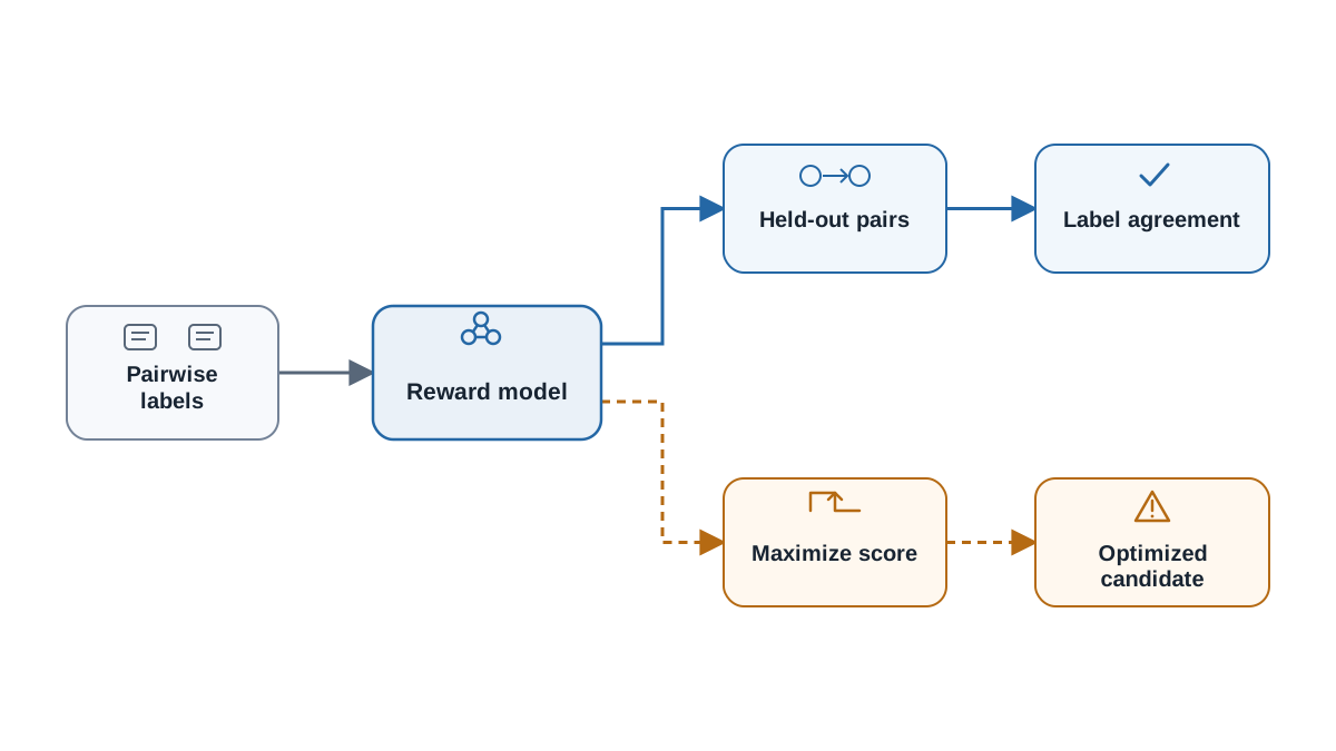
Accuracy answers "does it match my labels?" The question that actually matters is "what happens when something optimizes against it?"

Score a set of candidates the model never saw and rank them. Then read the top few by hand. Would a human agree? This is where proxy exploitation shows up. If your features include something correlated with preference but not the preference itself — length, verbosity, a spurious marker — the model will lean on it, because leaning on it reduces the training loss.

To see this in miniature, run a small optimization loop against the frozen reward model. Start from a random candidate vector, take gradient steps to maximize the score, and watch.

x = torch.randn(3, requires_grad=True)
opt = torch.optim.Adam([x], lr=0.1)
for step in range(200):
    opt.zero_grad()
    score = model(x)
    (-score).backward()
    opt.step()
print("optimized candidate:", x.detach().numpy())
print("score:", model(x).item())

The score climbs. Whether the resulting candidate is anything a human would want is a separate question — and usually the answer is no. That gap is reward hacking in miniature: the model is doing exactly what you asked, and what you asked was a proxy.

What is established: the model reproduces your labels on held-out contexts. What is not established: that maximizing it produces behavior anyone wants.

Where Ambiguity Enters the Data

Some of the model's uncertainty is inherited, not created by the optimizer.

Annotator disagreement is information about the objective, not just noise to average away. When two careful people disagree on a pair, that pair is underdetermined — and the model has no way to represent "I don't know" unless you built that in.

Pairs that differ on many dimensions at once make the preference uninterpretable. If candidate A is shorter, more accurate, and less polite than B, the label tells you which one won, not which dimension mattered. The model has to guess.

Try this: deliberately inject a contradictory pair — the same pair with the label flipped — and watch. The loss plateaus or the margin collapses. That is the data telling you the label set is inconsistent.

Practical rule: before blaming the model, check whether a careful human could reproduce your own labels. If they cannot, the model is not the problem.

One Experiment Worth Running

Add a spurious feature that correlates with the label in training but is absent or reversed in the held-out set. For example, if longer candidates happen to be preferred in your training pairs, add a length feature that is high for chosen and low for rejected — then flip it in the held-out data.

Predict before you run it: training accuracy stays high, held-out accuracy drops. Run it. Observe the gap. That gap is why reward models need distribution-matched evaluation, and why a benchmark score from a different distribution tells you almost nothing.

Optional second variant: train two models on disjoint halves of your data and compare their rankings on the same candidates. Where they disagree, the prediction is unreliable. Disagreement is a cheap uncertainty signal, and it costs you one extra training run.

What to Do With This

A reward model is a hypothesis about preference. The only way to know its scope is to test it on comparisons and behaviors it never saw — held-out pairs, order swaps, no-preference probes, and a small optimization loop that shows you what maximizing the proxy actually produces.

The next step is to put this audited reward inside a policy optimization loop. There, the gap between proxy and intent stops being a measurement problem and becomes an operational one: your policy will find every shortcut your reward model left open. The audit you just ran is the map of those shortcuts.