
What Can Pairwise Preferences Identify About an RL Reward Model?
Two reward models, same comparison data, different absolute scores—and both rank every trajectory identically. Neither is broken. The data never pinned…

Key topics
Two reward models, same comparison data, different absolute scores—and both rank every trajectory identically. Neither is broken. The data never pinned down a single reward function; it pinned down a family.
The Reward You Fit Is One of Many
You already know the pipeline: collect pairwise comparisons, fit a scalar reward surrogate, optimize a policy against it. The step that trips people up is the assumption buried in the middle. It is tempting to believe the model "learned the reward." What it actually learned is a function consistent with the observed comparisons—and there are usually many such functions.
Three things decide how much of the reward the data can actually pin down:
- The likelihood form. The preference model defines which reward transformations leave the data equally likely.
- The comparison graph. Which items were compared to which determines which reward differences are constrained.
- The modeling assumptions. The surrogate's expressiveness and the noise model cap what any amount of data can recover.
This article is a map of what pairwise preferences can and cannot identify. It is not about how to build the pipeline—that comes earlier. It is about what the signal determines once you have it.
Notation and the Bradley-Terry Likelihood
Let a trajectory segment be , and let be a learned scalar reward surrogate with parameters . A comparison gives a pair and a label , where means was preferred.
The Bradley-Terry model assumes each item has a latent positive strength , and the probability that beats is proportional to that strength:
Reparametrize with unbounded scores by setting . The ratio becomes a logistic function of the score gap:
where . The negative log-likelihood over a dataset of comparisons is:
Read that expression carefully. The loss depends only on the difference . Absolute reward levels never appear. The sigmoid is monotone in the gap, so a larger gap means a more confident preference—but the loss is blind to where the scores sit on the number line.
Knowledge check
Check your understanding
Answer this question before you continue.
Why Only Differences Are Identifiable
Take any fitted reward and add a constant to every score. The difference is unchanged:
The likelihood is identical. So is the gradient. So is every prediction the model makes. The reward is identified up to an additive constant—the data cannot distinguish from for any .
This is not a training bug or a regularization artifact. It falls directly out of the logistic form. In multi-expert or trust-weighted settings, the ambiguity widens: the likelihood can be invariant to a global affine reparameterization, where rewards are rescaled and shifted while trust parameters absorb the inverse scaling.
The practical consequence is blunt: absolute reward values are meaningless. Only relative ordering and the size of gaps carry information. If you compare raw scores across two training runs, you are reading noise dressed as signal.
Common mistake: Treating a reward of 3.7 as "better" than a reward of 2.1 from a different run. Without a shared normalization, those numbers live in different coordinate systems.
One boundary worth stating: this equivalence class is a property of the logistic preference model. Other preference models—regret-based, tie-aware, or strength-aware variants—can have different or narrower ambiguity. Do not generalize the additive-shift result to every preference framework.
Knowledge check
Check your understanding
Answer this question before you continue.
What the Comparison Graph Determines
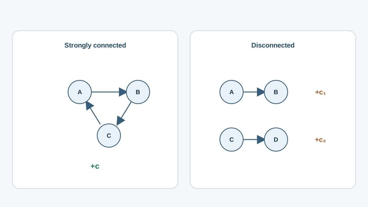
Build a directed graph: items are nodes, and each observed comparison is an edge from to . The structure of this graph decides which reward differences the data constrains.
In the standard finite Bradley-Terry setting, the relevant condition is strong connectivity of this directed graph: you can travel from any item to any other along the direction of observed wins. Under that condition, the fitted utilities are unique up to a single additive constant—every pairwise difference is pinned down relative to every other, and the equivalence class collapses to one degree of freedom. This is a statement about the fitted optimum, not about exact recovery: with finite noisy comparisons you are still estimating those differences from samples, so statistical uncertainty sits on top of the structural result.
Break strong connectivity and the guarantee breaks with it. Suppose your data splits into two clusters with no comparisons bridging them in either direction. Within each cluster, differences are constrained. Across clusters, nothing is. The model can assign cluster A an average reward of 10 and cluster B an average of -10, or swap those values, and the likelihood does not change. Each connected component carries its own free offset.
This is why coverage beats volume. A million comparisons inside one region of state-action space tells you almost nothing about a region the policy will actually visit. The limiting factor is not dataset size—it is whether the comparison graph reaches the places that matter.
Knowledge check
Check your understanding
Answer this question before you continue.
Assumptions That Do the Heavy Lifting
The identifiability results above are conditional. Each one rests on assumptions that fail in practice.
| Assumption | What it buys | What breaks when it fails |
|---|---|---|
| Preferences follow a logistic/Bradley-Terry form | The clean additive-shift equivalence class | Misspecification biases the inferred reward even with infinite data |
| Preferences are consistent, noise is well-behaved | The likelihood is the right objective | Ties, intransitivity, and annotator disagreement violate the model |
| The surrogate can represent the true reward | Identification is possible in principle | Function-approximation limits cap what any data can recover |
| Comparisons cover the relevant region | Identification is global | Sparse or clustered data yields only local identification |
The first assumption deserves emphasis. If human preferences systematically deviate from the logistic form—say, because annotators are more confident than the model assumes—then the fitted reward converges to the wrong function. More data does not fix a wrong model. It just makes you more confident in the wrong answer.
Note: Misspecification and ambiguity are different failure modes. Ambiguity means the data admits many rewards. Misspecification means the data admits the wrong one.
Knowledge check
Check your understanding
Answer this question before you continue.
A Small Numerical Walkthrough
Three items, , , , with observed preferences and . Consider two reward assignments:
- Assignment 1: , ,
- Assignment 2: , ,
For the pair , Assignment 1 gives a gap of , so . Assignment 2 gives a gap of , so . Identical. The same holds for : both assignments produce a gap of and the same probability. The likelihoods match exactly. The two assignments are in the same equivalence class—they differ only by the shared shift .
That example shows additive invariance, but it does not yet show the freedom that disconnected components create. For that, split the data into two clusters with no bridging comparison. Cluster 1 contains , so it constrains . Cluster 2 contains , so it constrains . Nothing connects the two clusters. Now shift every score in Cluster 1 by and leave Cluster 2 untouched. Every observed gap is preserved, so the likelihood is unchanged. The model can place Cluster 1's rewards far above Cluster 2's, or far below, and the data cannot object. Each component carries its own free offset.
An isolated item is the extreme case of this. Add item with no comparisons at all. Its reward appears in no difference term, so the loss is completely flat in . The model can set to any value—, —and the training loss does not move. is unconstrained, not because the model failed, but because the data said nothing about it.
Scale that up: replace the disconnected cluster with an entire region of state-action space your policy will explore, and you have a reward model that is confidently wrong exactly where it matters.
What This Means for Interpreting a Reward Model
Translate the theory into reading rules:
- Read differences, not absolute scores. Normalize rewards before comparing across runs. If you must report a single number, report a gap.
- High training accuracy is not identification. A model can fit every observed edge perfectly while leaving large regions of reward space unconstrained. Accuracy measures fit on the data you have, not coverage of the space you need.
- Ambiguity propagates into the policy. If a region's reward is unconstrained, policy optimization will find and exploit it. This is one mechanism behind reward hacking from unconstrained regions—the policy is not gaming the reward, it is filling in a blank the data left open.
- Graph coverage is one audit dimension, not a certificate. Dense, strongly connected comparisons over the policy-relevant region tell you the structural support is there. They do not tell you the model form is right, the noise assumptions hold, or the surrogate can represent the true reward. Those require held-out prediction checks and model diagnostics.
The question to ask before trusting any fitted reward is not "how accurate is it?" but "what does its comparison graph cover, and which equivalence class does it leave open?"
Where the Guarantees Stop
Identifiability results are conditional on the model class and the comparison structure. They are not universal laws. Finite data adds statistical uncertainty on top of structural ambiguity—even a strongly connected graph leaves you estimating differences from noisy samples. Multi-expert and trust-weighted settings introduce additional scaling ambiguities that require their own connectedness conditions to resolve.
An open direction worth watching: designing query sets that maximize identifiability rather than raw accuracy. The current default—collect comparisons wherever they are cheap—optimizes the wrong objective if your goal is a reward you can actually interpret.
Your Next Step
Before you trust a reward model, audit it. Take held-out comparisons the model never trained on, and check whether its predicted differences match the observed labels. Then map the comparison graph: are there clusters with no bridging edges in either direction? Those clusters are where your reward model is guessing, and where your policy will eventually go looking for loopholes. The audit tells you whether the identified structure is real or an artifact of where you happened to collect data.
Knowledge check
Final check
Finish the article by checking the ideas you just learned.
References
Build a stronger RL mental model
Use structured resources to connect equations, algorithms, and observable agent behavior.


