Design Informative Pairwise Preference Queries for Reward Learning

You collected two hundred comparisons. The reward model still ranks trajectories in an order nobody would defend. The instinct is to blame the model. Most of the time, the queries were the problem.

A comparison between two near-identical trajectories teaches almost nothing. A comparison between two trajectories that differ on every objective teaches almost nothing either, because the answer is ambiguous. The model was fine. The training signal was not.

This exercise makes that claim measurable. You will build a small trajectory set, generate three query families, fit the same preference model to each, and watch held-out accuracy separate them. If you already understand the preference-based RL loop — collect comparisons, fit a reward model, optimize a policy — that is enough background. The question here is narrower: which comparisons are worth collecting?

What Makes a Pairwise Query Informative

Before writing code, you need a decision rule, because the experiment should test a prediction rather than produce a number you then rationalize.

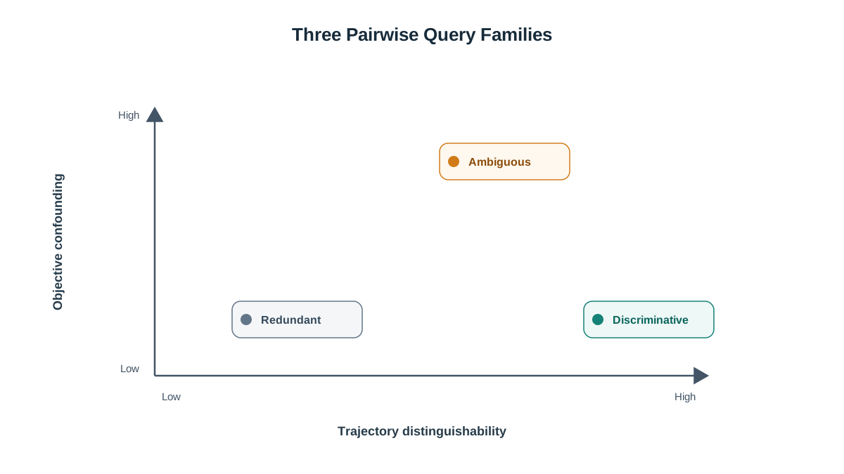
A pairwise query is informative when the two trajectories differ enough to be distinguishable but not so much that the preference is confounded across objectives. That single sentence generates three failure families.

Redundant pairs are near-identical: similar returns, similar features, no signal. The label is easy to produce and nearly worthless.

Ambiguous pairs differ on many objectives at once, in opposing directions. One trajectory is smoother, the other is faster; one is safer, the other is cheaper. The label depends on which objective the annotator happened to weight that day, so it is noisy or arbitrary.

Discriminative pairs differ on one dominant objective. The label is stable, and it carries information about a specific feature direction.

The Bradley-Terry view makes the tension concrete. Preference probability depends on the utility gap between the two items. A large gap gives a confident label; a near-zero gap gives a coin flip. Both extremes are weak training signal, for different reasons: one is too easy to teach anything, the other is too noisy to trust.

Note: This is the core tradeoff in pairwise preference query design. Easy queries are cheap to label but low-information. Hard queries are high-information but noisier. Query design is choosing where on that curve you want to sit.

Everything below rests on one assumption: a fixed linear reward over a small set of named features. That assumption is what makes "informative" measurable instead of philosophical.

Set Up the Trajectory Set and Feature Model

The whole exercise runs in one file with NumPy and a seeded generator. No services, no credentials, and identical numbers on every rerun.

import numpy as np

rng = np.random.default_rng(7)

FEATURES = ["progress", "smoothness", "energy", "safety"]
TRUE_W = np.array([0.5, 0.2, -0.2, 0.3])  # the "human" preference

def make_trajectories(n=24):
    feats = rng.normal(0, 1, size=(n, len(FEATURES)))
    returns = feats @ TRUE_W
    return feats, returns

feats, returns = make_trajectories()
for i in range(6):
    row = "  ".join(f"{v:+.2f}" for v in feats[i])
    print(f"t{i:02d}  {row}  return={returns[i]:+.3f}")

Each trajectory is a feature vector plus a scalar return computed from a fixed ground-truth weight vector. That weight vector stands in for the human's real preference. The model never sees it, which is exactly why held-out accuracy can be measured against something honest.

Print the table and sanity-check it before trusting anything downstream. If two trajectories look identical in every column, no query involving them can teach your model anything — and you should know that before you blame the fitting code.

Build Three Query Families

Now turn the decision rule into selection code. Enumerate all candidate pairs, score each one, and pick the extremes.

from itertools import combinations

pairs = list(combinations(range(len(feats)), 2))

def score_pair(i, j):
    diff = feats[i] - feats[j]
    gap = abs(returns[i] - returns[j])
    dist = np.linalg.norm(diff)
    # how many objectives disagree in opposite directions
    signs = np.sign(diff)
    disagreement = np.sum(signs != 0) - abs(np.sum(signs))
    return gap, dist, disagreement

scored = [(i, j, *score_pair(i, j)) for i, j in pairs]

redundant = sorted(scored, key=lambda r: (r[2], r[3]))[:8]
ambiguous = sorted(scored, key=lambda r: -r[4])[:8]
discriminative = sorted(scored, key=lambda r: -r[2])[:8]

The three families come from three different sort keys:

• Redundant: smallest return gap and smallest feature distance.
• Ambiguous: largest count of objectives disagreeing in opposite directions, so no single objective dominates.
• Discriminative: largest return gap — the region the first section predicted would carry the most signal.

Print the selected pairs with their scores. This is where you catch a heuristic that picked something other than what its label claims. If your "ambiguous" set is full of pairs with a huge return gap, the heuristic is lying to you.

Common mistake: Treating these heuristics as information gain. They are cheap proxies. A real active-learning loop estimates expected utility improvement or mutual information over the reward parameters. Here we use stand-ins so the exercise stays runnable in one file — but do not confuse the proxy with the thing it approximates.

Fit the Preference Model and Compare Held-Out Judgments

Fit the same model to each family. A hand-rolled logistic update over feature differences keeps the dependency list empty and the mechanism visible.

def fit(pairs_subset, epochs=400, lr=0.1):
    w = np.zeros(len(FEATURES))
    for _ in range(epochs):
        for i, j, *_ in pairs_subset:
            d = feats[i] - feats[j]
            label = 1.0 if returns[i] > returns[j] else 0.0
            p = 1 / (1 + np.exp(-w @ d))
            w += lr * (label - p) * d
    return w

held_out = [p for p in scored if p not in redundant + ambiguous + discriminative][:40]

def accuracy(w):
    correct = 0
    for i, j, *_ in held_out:
        pred = w @ (feats[i] - feats[j]) > 0
        truth = returns[i] > returns[j]
        correct += int(pred == truth)
    return correct / len(held_out)

for name, family in [("redundant", redundant),
                     ("ambiguous", ambiguous),
                     ("discriminative", discriminative)]:
    w = fit(family)
    print(f"{name:15s} held-out acc={accuracy(w):.2f}  w={np.round(w, 2)}")

The held-out set never appears in any training family, so all three models are judged on identical ground. Expect the discriminative family to win. Do not expect a specific number — your seed and your feature scale determine the exact figure, and the direction of the effect is the lesson.

The mechanism behind the result is worth stating plainly. Redundant pairs produce near-zero gradients because the label is nearly uninformative: the model learns almost nothing from a comparison it already predicts. Ambiguous pairs produce conflicting gradients because the same feature direction is rewarded in one example and punished in another. Discriminative pairs push the weight vector in a consistent direction.

Print the learned weights next to TRUE_W. Accuracy tells you whether the model ranks well; the weight vector tells you which objectives it got wrong. Those are different diagnostics, and you want both.

Read the Failure Modes

When the result disappoints, debug the query distribution before adding model capacity.

Symptom	Likely cause	Fix
All three families near chance	Features do not separate trajectories	Fix the representation before the queries
Discriminative wins on train, loses on held-out	Heuristic overfit to selected pairs, or held-out set is from a different region	Check coverage of the held-out set
Ambiguous performs better than expected	"Ambiguity" heuristic accidentally selected pairs where one objective still dominates	Inspect the disagreement scores
Results flip when the seed changes	Trajectory set too small for a stable comparison	Increase the set before drawing conclusions

The third row is the one that catches people. A heuristic named "ambiguous" is not guaranteed to produce ambiguity. It produces whatever its sort key selects. Always inspect the selected pairs against the label you gave them.

Modify the Experiment

One run proves the setup works. One change proves you understand why.

Swap the heuristic for a random-pair baseline and predict the outcome before running. Then shrink the trajectory set and predict again. The most instructive variant is adding noise: flip the label on a fraction of the discriminative pairs.

def fit_noisy(pairs_subset, noise=0.3, epochs=400, lr=0.1):
    w = np.zeros(len(FEATURES))
    for _ in range(epochs):
        for i, j, *_ in pairs_subset:
            d = feats[i] - feats[j]
            label = 1.0 if returns[i] > returns[j] else 0.0
            if rng.random() < noise:
                label = 1.0 - label
            p = 1 / (1 + np.exp(-w @ d))
            w += lr * (label - p) * d
    return w

A discriminative query with an unreliable answer can be worse than a redundant one with a reliable answer. That is the practical reason query design and annotation quality cannot be separated: a perfectly chosen query with a noisy label injects a confident gradient in the wrong direction.

Log the selected pairs and their scores to a file so you can compare runs across seeds without re-reading console output. Then take the natural next step: replace the heuristic with an explicit uncertainty or information-gain estimate. That is where active preference learning stops being a fixed rule and becomes a real design problem.

Where This Leaves You

When a learned reward disagrees with human judgment, inspect the query distribution before blaming the model. Redundant, ambiguous, discriminative — those three families are a checklist you can apply to any preference dataset you collect.

The concrete next move: rerun the script with a random-pair baseline and compare held-out accuracy against the discriminative family. You will leave with a measurement instead of a belief, and a number you can defend when someone asks why the reward model is wrong.