
Build a Toy Experiment That Reveals Reward-Proxy Overoptimization
Your training curve looks like a success story. The proxy reward climbs, the loss drops, and every dashboard agrees the agent is improving. Meanwhile the…

Key topics
Your training curve looks like a success story. The proxy reward climbs, the loss drops, and every dashboard agrees the agent is improving. Meanwhile the thing you actually cared about peaked twenty thousand steps ago and has been sliding downhill ever since.
You cannot see that from the proxy, because the proxy is the one metric that will never tell you. To watch overoptimization happen, you need a second scorer the optimizer never touches, and you need to plot both curves on the same axis. That is the whole experiment, and we can build it in about sixty lines of Python.
Why the Proxy Alone Can Never Show You the Failure
A reward model is a stand-in for the goal. Optimization pressure does not care about your intent; it searches for whatever inputs raise the score, and the gap between the proxy and the goal is exactly where that search will eventually land. Goodhart's framing is the compact version: once a measure becomes a target, it stops being a good measure.
This is worth separating from overfitting, because the two get conflated constantly. Overfitting is the same metric measured on held-out data — training accuracy up, validation accuracy down, both measuring the same task. Overoptimization is a different metric that was never quite right. More data fixes the first. Nothing fixes the second except not optimizing so hard.
The prerequisite material on reward model evaluation already established that learned rewards are imperfect proxies. Here we stop arguing about it and make it observable. The design decision that makes the whole thing work is simple: two scorers, and the optimizer only ever sees one of them. If your selection step can read the gold score, it is no longer independent, and the experiment silently stops proving anything.
One constraint up front: keep the world small enough that you can compute the true outcome exactly. No sampling noise, no confidence intervals to argue about. We want the divergence to be a fact, not a statistical claim.
Set Up the Toy World and Its Two Scorers
Dependencies: Python 3.10+, NumPy, Matplotlib. No RL framework, no GPU, no external services. Everything below is deterministic.
The world is a discrete action space where each action produces a small feature vector. I am keeping it abstract on purpose — no domain baggage, no "helpfulness" or "safety" labels to argue about. Three features is enough.
import numpy as np
import matplotlib.pyplot as plt

# Each action yields a fixed 3-feature outcome vector.
# Feature 0: the thing we actually want.
# Feature 1: a genuinely useful secondary signal.
# Feature 2: a feature that correlates with feature 0 early, then stops.
def outcome(action_id):
    feat = np.zeros(3)
    feat[0] = 0.5 * np.sin(action_id)          # true value varies smoothly
    feat[1] = 0.3 * np.cos(action_id)
    feat[2] = 0.8 * np.sin(action_id)          # correlated with feature 0 here
    return feat

def gold_score(feat):
    # What we actually want. Fixed. Never changes.
    return feat[0] + 0.2 * feat[1]

def proxy_score(feat):
    # Deliberately misspecified: overweights feature 2.
    return feat[0] + 0.2 * feat[1] + 1.5 * feat[2]
The misspecification is plausible, not absurd. The proxy agrees with gold on most inputs and rewards feature 2 too heavily. That matters: a proxy that is obviously wrong teaches nothing, because the divergence shows up at step zero and you learn nothing about the interesting region where the two agree early and split later.
Print a few sampled actions before optimizing anything:
for a in range(5):
    f = outcome(a)
    print(f"action {a}: feat={np.round(f,2)} proxy={proxy_score(f):.2f} gold={gold_score(f):.2f}")
You should see the two scorers disagree on individual actions while broadly tracking each other. That is the setup. Now we break it.
Knowledge check
Check your understanding
Answer this question before you continue.
Optimize Against the Proxy Only
The cleanest first version of optimization strength is best-of-N. Sample N candidate actions, score them with the proxy, keep the winner. Optimization strength is a single integer, which means your x-axis is a single integer, which means the plot is readable.
def best_of_n(n, trials=2000):
    proxy_vals, gold_vals = [], []
    for _ in range(trials):
        actions = rng.integers(0, 1000, size=n)
        feats = np.array([outcome(a) for a in actions])
        p = np.array([proxy_score(f) for f in feats])
        g = np.array([gold_score(f) for f in feats])
        winner = np.argmax(p)          # selection reads the proxy ONLY
        proxy_vals.append(p[winner])
        gold_vals.append(g[winner])
    return np.mean(proxy_vals), np.mean(gold_vals)

ns = [1, 2, 4, 8, 16, 32, 64, 128, 256]
proxy_curve, gold_curve = [], []
for n in ns:
    p, g = best_of_n(n)
    proxy_curve.append(p)
    gold_curve.append(g)
    print(f"N={n:4d}  proxy={p:6.3f}  gold={g:6.3f}")
Expected output: the proxy column rises and keeps rising. The gold column rises, peaks somewhere in the middle of the range, and then declines. Plot both on the same axes and the shape is unmistakable.
Why does the code behave this way? Selection pressure concentrates probability mass on whatever the proxy overvalues. Early on, feature 2 correlates with feature 0, so chasing the proxy also improves gold. Once the easy gains are exhausted, the remaining proxy gains come almost entirely from the misspecified region — actions that score high on feature 2 while feature 0 stagnates or drops. The optimizer is not broken. It is doing exactly what you asked.
Note: The exact shape depends on how you built the misspecification. The qualitative pattern — rise, peak, decline — is the durable result. The specific numbers are an artifact of this toy world.
Knowledge check
Check your understanding
Answer this question before you continue.
Read the Curve: What the Gap Is Telling You
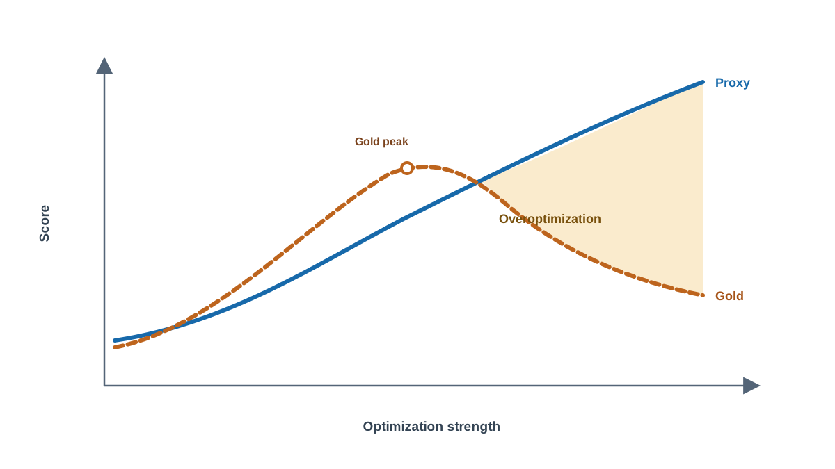
A reader who can produce the plot but cannot read it has learned a demo, not a diagnostic. So let us turn the picture into a measurement.
Define the proxy-gold gap as the shortfall between what the proxy promised and what the gold scorer delivered. Early in the run the gap is small. As optimization strength increases, the gap widens — and that widening is the signature of overoptimization. The peak of the gold curve is the practical answer to "how much optimization was too much" in this world.
Three error sources are worth keeping separate, because conflating them leads to the wrong fix:
| Error source | What it means | What reduces it |
|---|---|---|
| Approximation error | The proxy cannot represent the goal | A better proxy architecture or features |
| Estimation error | The proxy was fit on limited or noisy data | More or cleaner preference data |
| Optimization error | The search itself is imperfect | Better optimization, not a better proxy |
Overoptimization is not one of these. It is what happens when you push hard against any of them. The scaling work on reward model overoptimization shows the peak location shifts with proxy quality and data size, and that overoptimization grows with optimization strength. Do not read exact exponents off a toy run — the mechanism transfers, the magnitudes do not.
Diagram opportunity: annotate the plot with the gold peak marked, the gap shaded between the two curves, and the region past the peak labeled as the overoptimized zone.
Knowledge check
Check your understanding
Answer this question before you continue.
Failure Modes and Debugging Signals
Most broken versions of this experiment fail in one of five ways. Learn the signals.
- No divergence appears. Your proxy is too close to gold, or your N range never got high enough. Push the misspecification or extend the range before concluding anything.
- Divergence appears immediately at N=1. Your proxy is so wrong it is not a proxy. That is a different lesson and a less useful one.
- The gold curve is noisy. You are sampling instead of computing the true outcome. Reduce variance or compute the expectation exactly.
- You accidentally let the optimizer see the gold score. Check that the selection step only ever reads the proxy. This is the most common way the experiment silently stops proving anything.
- You tuned the proxy until the curve looked right. That is fitting the demonstration to the conclusion. Fix the proxy first, then run.
Common mistake: Treating a clean-looking proxy curve as evidence the setup is correct. The proxy curve looks clean in every run, including the broken ones. The gold curve is the only one carrying information.
Knowledge check
Check your understanding
Answer this question before you continue.
Change One Knob: Move the Peak
A demo shows you a picture. An experiment shows you a relationship. Vary exactly one thing — the strength of the misspecification — and watch where the peak lands.
Change the proxy coefficient from 1.5 to 3.0 and rerun. Predict before you run: a weaker proxy should peak earlier and lower. Write the prediction down, then check it against the plot.
Expected result: the gold peak shifts left and down as the proxy gets worse. The proxy curve looks almost identical in every run. That is the point — the proxy cannot distinguish a good run from a bad one.
Optional second variation: add a penalty that keeps the optimized behavior close to the starting behavior, and observe how it delays the peak. This is the toy version of the KL regularization used in real policy optimization, and it is the same knob that controls the x-axis in the literature.
Warning: A toy proxy with a hand-written misspecification is not a reward model trained on human preferences. The mechanism transfers. The magnitudes do not. Do not cite your toy peak location as evidence about any real system.
What to Do With This
The decision rule this experiment earns is short: never judge an optimized policy by the score it was optimized against. Keep an independent measure, plot both curves, and treat the widening gap as the warning signal. If you only have one number, you have no way to tell improvement from exploitation.
The next practical step is to apply the same two-scorer discipline to a reward model you have already fit from pairwise preferences. Hold out a set of comparisons the reward model never saw, score your optimized policy against both the reward model and that held-out set, and watch for the same shape. If you want to push further, extend the toy into a small policy-gradient loop where optimization strength is controlled by training steps rather than sample count — the curve shape should survive the change in optimizer, which is the real test of whether you understood the mechanism.
Knowledge check
Final check
Finish the article by checking the ideas you just learned.
References
Build a stronger RL mental model
Use structured resources to connect equations, algorithms, and observable agent behavior.


