Diagnose Simulator-to-Deployment Mismatches From Paired Traces

Your policy scored well in simulation. On the target system, it behaves differently. All you have is two logs of the same episode — one from each system — and they disagree. That disagreement is evidence, but it is not a verdict. This exercise gives you a repeatable way to narrow which mismatch family is most likely responsible, using only Python and the traces themselves.

We will load paired traces, run four targeted checks in order, and read each output as a symptom that shrinks the search space. The deliverable is not a diagnosis. It is one concrete next test that can falsify your leading hypothesis.

What Paired Traces Can and Cannot Tell You

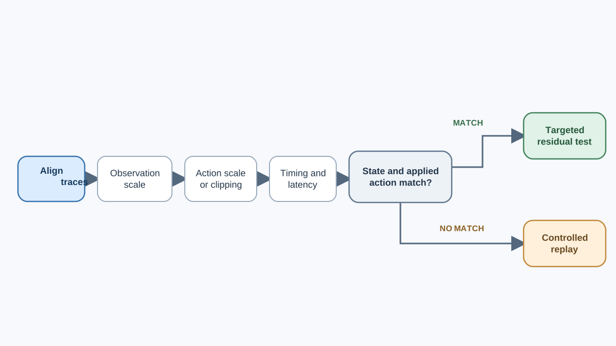
A paired trace is two aligned records of the same policy acting in two systems: the simulator and the target. Same checkpoint, same episode structure, two different worlds.

Trace comparison narrows the symptom space. It does not prove causation, and it does not produce a transfer score. If you finish this exercise and announce "the gap is dynamics," you have overread the evidence. What you can honestly say is: "After correcting for observation scaling and action clipping, the residual disagreement in next-state transitions is consistent with a dynamics mismatch, and the next test should isolate that."

Four mismatch families are in scope:

• Observation scaling
• Action clipping or scaling
• Timing or latency
• Transition dynamics

Alignment is the precondition for all four. If timestamps or step indices do not line up, every later check is suspect. Fix alignment first, or the rest is noise dressed as signal.

If you have already worked through why policies break outside the simulator, you know these mismatch sources exist. Here you learn to localize them from data.

The Exercise Setup and Trace Schema

You need Python 3 with numpy and pandas. No GPU, no external services, no credentials.

Two files: sim_trace.csv and target_trace.csv. Each is a sequence of records. The minimum fields per record:

Field	Meaning
step	Integer step index
timestamp	Wall-clock or monotonic time
obs	Observation vector (list or JSON)
action	Action vector the policy emitted
reward	Scalar reward
done	Episode termination flag

Optional but useful: obs_raw (pre-normalization observation), action_applied (post-clip action), and any latency measurement.

Note: Both traces must come from the same policy checkpoint. If they do not, the comparison is meaningless — you are comparing two different policies, not two systems.

To make this exercise runnable without your own logs, here is a small deterministic fixture. It builds a two-dimensional observation, a one-dimensional action, and a target system that scales observations by 1.5, clips actions at 0.5, and adds a small dynamics offset. Run this first, then run the checks against the resulting DataFrames.

import numpy as np
import pandas as pd

rng = np.random.default_rng(0)
n = 40

# Simulator: clean dynamics
sim_obs = np.cumsum(rng.normal(0, 0.1, size=(n, 2)), axis=0)
sim_act = np.clip(rng.normal(0, 0.4, size=(n, 1)), -1.0, 1.0)
sim_ts = np.arange(n) * 0.05

# Target: observation scale 1.5, action clipped at 0.5, small dynamics offset
tgt_obs = sim_obs * 1.5 + rng.normal(0, 0.01, size=(n, 2))
tgt_act = np.clip(sim_act, -0.5, 0.5)
tgt_ts = np.arange(n) * 0.05 + 0.01  # constant 10 ms lag

sim = pd.DataFrame({
    "step": np.arange(n),
    "timestamp": sim_ts,
    "obs": list(sim_obs),
    "action": list(sim_act),
    "reward": np.zeros(n),
    "done": False,
})
target = pd.DataFrame({
    "step": np.arange(n),
    "timestamp": tgt_ts,
    "obs": list(tgt_obs),
    "action": list(tgt_act),
    "action_applied": list(tgt_act),
    "reward": np.zeros(n),
    "done": False,
})

print(sim.shape, target.shape)
print(sim.head(3))

Expected output: (40, 6) (40, 6), followed by the first three rows. If your own traces differ by more than a few steps in row count, check alignment before continuing.

Check 1: Observation Scaling

Compare per-dimension observation statistics between the two traces.

sim_obs = np.stack(sim["obs"].values)
tgt_obs = np.stack(target["obs"].values)

stats = pd.DataFrame({
    "sim_mean": sim_obs.mean(axis=0),
    "tgt_mean": tgt_obs.mean(axis=0),
    "sim_std": sim_obs.std(axis=0),
    "tgt_std": tgt_obs.std(axis=0),
})
stats["mean_ratio"] = stats["tgt_mean"] / (stats["sim_mean"] + 1e-9)
stats["std_ratio"] = stats["tgt_std"] / (stats["sim_std"] + 1e-9)
print(stats)

With the fixture, both dimensions show std_ratio near 1.5 — the scale factor we injected. Read the ratios, not the raw values. A dimension whose std_ratio is near 1 but whose mean_ratio is far from 1 suggests a constant offset. A dimension where both ratios drift together suggests a scale factor. These imply different fixes and different next tests.

Common mistake: Reading mean_ratio as a scale signal when the simulator mean is near zero. A ratio against a near-zero denominator explodes. Trust std_ratio for scale, and treat mean_ratio as a lead only when the simulator mean is meaningfully away from zero.

Failure signal: a dimension that saturates at a bound in the target trace but not in simulation. That is a normalization or unit mismatch, and it will poison every downstream comparison.

Check 2: Action Clipping and Scaling

Compare the action the policy emitted against the action actually applied.

sim_act = np.stack(sim["action"].values)
tgt_act = np.stack(target["action"].values)

if "action_applied" in target.columns:
    tgt_applied = np.stack(target["action_applied"].values)
    delta = tgt_applied - tgt_act
    print("Mean |emitted - applied|:", np.abs(delta).mean(axis=0))
    print("Fraction at bound:", (np.abs(tgt_applied) >= 0.49).mean(axis=0))

With the fixture, the fraction at bound is well above zero because the target clips at 0.5 while the simulator allows up to 1.0. Look for mass piled at the action-space bounds in the target trace. That is the signature of clipping. Clipping flattens the tails of the distribution; scaling shifts and stretches the whole thing. They look similar in a histogram and demand different fixes.

Failure signal: identical policy outputs producing different applied actions across the two traces. That means the target system is altering the policy's intent before it reaches the actuators.

Common mistake: Assuming the simulator and target share the same action bounds and units. They often do not, and the mismatch hides in the gap between emitted and applied.

Check 3: Timing and Latency

Compare inter-step intervals and the delay between observation and applied action.

sim_dt = np.diff(sim["timestamp"].values)
tgt_dt = np.diff(target["timestamp"].values)

print("Sim dt: mean=%.4f std=%.4f" % (sim_dt.mean(), sim_dt.std()))
print("Target dt: mean=%.4f std=%.4f" % (tgt_dt.mean(), tgt_dt.std()))

# Constant offset between clocks
offset = target["timestamp"].values[0] - sim["timestamp"].values[0]
print("Clock offset: %.4f" % offset)

With the fixture, both dt means are 0.05 and the clock offset is 0.01. A consistent lag in the target trace shifts every downstream comparison. Correct for it before reading the other checks — subtract the offset from the target timestamps, or align by step index if the offset is constant. Watch for clock or timestamp inconsistencies that make alignment look correct when it is not. If the target timestamps come from a different clock source, the intervals may be plausible while the alignment is wrong.

Latency can present as a dynamics mismatch if you skip this check first. The same action sequence produces different state transitions purely as a function of delay.

Failure signal: the target trace shows a systematic lag that grows or stays constant, and the state divergence tracks that lag rather than the action sequence.

Check 4: Transition Dynamics Mismatch

This check isolates disagreement that survives the first three. The claim is narrow: given the same previous state and the same applied action, compare the resulting next state. If the previous states do not match, you are not comparing dynamics — you are comparing two different trajectories.

# Align by step index after correcting for timing
n = min(len(sim), len(target))
sim_obs = np.stack(sim["obs"].values)[:n]
tgt_obs = np.stack(target["obs"].values)[:n]
sim_a = np.stack(sim["action"].values)[:n]
tgt_a = np.stack(target["action"].values)[:n]

# Require both previous states and applied actions to match closely
state_match = np.linalg.norm(sim_obs[:-1] - tgt_obs[:-1], axis=1) < 0.05
action_match = np.linalg.norm(sim_a[:-1] - tgt_a[:-1], axis=1) < 0.01
mask = state_match & action_match

print("Comparable transitions:", mask.sum(), "of", n - 1)

if mask.sum() > 0:
    residual = np.linalg.norm(
        sim_obs[1:][mask] - tgt_obs[1:][mask], axis=1
    )
    print("Residual next-state disagreement: mean=%.4f std=%.4f"
          % (residual.mean(), residual.std()))
else:
    print("No comparable transitions. Trajectories diverged before dynamics "
          "could be isolated.")

With the fixture, the observation scale factor of 1.5 means state_match fails almost everywhere. That is the correct outcome: the traces are not comparable at the transition level until you correct the observation scaling from Check 1. Re-run after dividing tgt_obs by 1.5 and the mask will populate.

This is the weakest-evidence check. It is easy to attribute to dynamics what is actually an upstream artifact. Only trust it after observation, action, and timing are accounted for. If the mask is empty, the honest conclusion is residual trajectory disagreement, not dynamics mismatch — and the next test is a controlled replay, not a dynamics model change.

Look for systematic drift versus noise. A consistent bias suggests a modeling gap. Scatter suggests stochasticity or measurement error.

Failure signal: divergence that grows with episode length rather than appearing immediately. That pattern points at accumulated dynamics error, not a one-time offset.

Reading the Outputs Without Overclaiming

Each check produces a symptom, not a root cause. Two checks can fire for one underlying problem. Rank findings by how much of the trace they explain, not by how easy they were to compute.

State what is observed, what is inferred, and what remains untested. A clean check is evidence of absence only within the range the trace covers. If your episode never pushed the action into the upper bound, a clean clipping check tells you nothing about what happens when it does.

Do not convert any of this into a single transfer score. The traces do not support one.

Choosing Your Next Validation Test

Map each surviving symptom to a targeted test:

• Observation scaling → replay with corrected normalization
• Action clipping → re-run with matched action bounds
• Timing → inject a controlled delay into the simulator
• Dynamics → isolate one transition and compare against a hand-computed expectation

Change one factor at a time so the next trace pair is interpretable. Prefer the test that can falsify your leading hypothesis fastest. Record the predicted outcome before running it, so the result teaches you something either way.

If two hypotheses survive, design a test that separates them rather than testing both at once.

Modify the Exercise: Add a Fifth Check

Add a reward-consistency check: same state and action should yield the same reward in both systems. Or add a termination-condition check: episodes ending at different points for the same behavior.

Both extensions reuse the alignment and comparison machinery you already built. Reward and termination mismatches are easy to miss when you only compare observations and actions, and they can silently reshape the learning signal even when the dynamics look correct.

When traces disagree, run the four checks in order. Treat each output as a symptom that narrows the search space. Pick the single next test that can falsify your leading hypothesis.

The natural follow-on is to turn this into a small reusable script you can point at your own simulator and target logs. A clean trace pair is evidence about the range it covers — not a certificate of transfer.