Deriving Soft Bellman Equations From the Entropy-Regularized Objective

You add an entropy bonus to your objective, and the whole value structure shifts under your feet. The max in the Bellman backup becomes a log-sum-exp. The greedy policy becomes a softmax. The temperature stops acting like a learning-rate knob and starts acting like a price. None of that is a bug in your implementation. It is what happens when entropy moves inside the return instead of sitting beside it.

This article derives that shift. I assume you already have the standard Bellman expectation and optimality relationships and the likelihood-ratio policy-gradient estimator in hand. Here I derive only the delta: where the entropy term enters the objective, how it propagates into the value definitions, why the optimality backup becomes a log-sum-exp, and what the temperature actually means.

Why the Entropy Term Cannot Stay Outside the Value Function

The weak model most people carry is this: entropy is an exploration bonus. You keep your value functions exactly as they were, and you add a bonus gradient term to the policy update. The bonus nudges the policy toward diversity early in training, then fades as the policy converges.

That model works for exactly one job — keeping a policy from collapsing onto a premature deterministic solution while the critic is still wrong. It fails the moment you ask what the optimal policy looks like under the augmented objective. If entropy is part of the return, then the value of a state must already account for the entropy the policy will collect in the future. You cannot compute a value that ignores a term that appears in every future step's return.

So the reframe: entropy regularization changes the return definition, and therefore changes the Bellman operator itself. The value functions are not unchanged. They are redefined.

Here is the notation I will use throughout. State $s \in \mathcal{S}$, action $a \in \mathcal{A}$, transition kernel $P(s' \mid s, a)$, reward $r(s, a)$, discount $\gamma \in [0, 1)$, policy $\pi(a \mid s)$, and temperature $\alpha > 0$. The temperature is a scalar weight on the entropy term. It is not a property of the environment.

Writing the Entropy-Regularized Objective

The augmented per-step return adds a temperature-weighted entropy term to the reward:

$$\tilde{r}(s, a) = r(s, a) + \alpha \, \mathcal{H}\big(\pi(\cdot \mid s)\big)$$

where $\mathcal{H}(\pi(\cdot \mid s)) = -\sum_a \pi(a \mid s) \log \pi(a \mid s)$ is the Shannon entropy of the policy at state $s$. The full objective maximizes the expected discounted sum of $\tilde{r}$ over trajectories.

The general form replaces Shannon entropy with the KL divergence to a reference policy $p$:

$$\mathcal{H}\big(\pi(\cdot \mid s) \,\|\, p(\cdot \mid s)\big) = -\sum_a \pi(a \mid s) \log \frac{\pi(a \mid s)}{p(a \mid s)}$$

Shannon entropy is the special case where $p$ is uniform. The general form matters for derivations because it keeps the reference policy explicit, and because it is the form that survives when you want a policy to stay near a prior rather than spread uniformly.

State the assumptions before the algebra, because they are load-bearing:

• Finite action space. The closed-form log-sum-exp and Boltzmann policy below require a finite $\mathcal{A}$. Continuous actions lose the closed form.
• Finite return. Either episodic or discounted, so the sum of rewards and entropies is finite.
• Differentiable, strictly positive policy. A policy that assigns zero probability to an action makes $\log \pi$ unbounded, and the derivation breaks.

Common mistake: Treating the temperature as a property of the environment. It is a scalar you choose, and it sets the exchange rate between reward and stochasticity. Change it and you change the optimal policy, not just the learning dynamics.

Deriving the Soft Value Functions

Start from the entropy-augmented return and take the expectation under the policy. The soft state value is:

$$V^\pi(s) = \mathbb{E}_{\pi}\left[\sum_{t=0}^{\infty} \gamma^t \big(r(s_t, a_t) + \alpha \, \mathcal{H}(\pi(\cdot \mid s_t))\big) \,\Big|\, s_0 = s\right]$$

The soft action value is the same expectation conditioned on the first action:

$$Q^\pi(s, a) = r(s, a) + \gamma \, \mathbb{E}_{s' \sim P}\big[V^\pi(s')\big]$$

Notice what is absent from $Q^\pi$: the entropy term at the current step. The action $a$ is already chosen, so the current-step entropy does not depend on it. This is the single most common place readers expect a term that is not there. The entropy term attaches at the successor state, not the current action.

The relationship between soft $V$ and soft $Q$ follows from the definition of the expectation:

$$V^\pi(s) = \mathbb{E}_{a \sim \pi}\big[Q^\pi(s, a)\big] - \alpha \, \mathbb{E}_{a \sim \pi}\big[\log \pi(a \mid s)\big]$$

That is an expectation of $Q$ minus temperature times log-policy — not a plain expectation of $Q$. Compare it to the standard relationship $V^\pi(s) = \mathbb{E}_{a \sim \pi}[Q^\pi(s, a)]$ and you can see exactly which term was inserted and where.

A backup diagram makes the placement concrete. Draw the reward node and the successor value node as usual. Attach the entropy node at the successor state, hanging off the policy that selects the next action — not off the current action.

Deriving the Soft Bellman Equations

Substitute the soft $Q$ definition into the soft $V$ definition and expand one step. You get the soft Bellman expectation equation:

$$V^\pi(s) = \mathbb{E}_{a \sim \pi}\Big[r(s, a) + \alpha \, \mathcal{H}(\pi(\cdot \mid s)) + \gamma \, \mathbb{E}_{s' \sim P}\big[V^\pi(s')\big]\Big]$$

Now maximize the right-hand side over the policy. This is the key algebraic move. You are maximizing an expectation of $Q$ minus temperature times log-policy over the probability simplex:

$$\max_{\pi} \; \mathbb{E}_{a \sim \pi}\big[Q(s, a)\big] - \alpha \, \mathbb{E}_{a \sim \pi}\big[\log \pi(a \mid s)\big]$$

The solution is a Boltzmann distribution:

$$\pi^*(a \mid s) = \frac{\exp\big(Q(s, a) / \alpha\big)}{\sum_{a'} \exp\big(Q(s, a') / \alpha\big)}$$

and the resulting value is temperature times log-sum-exp:

$$V^*(s) = \alpha \log \sum_a \exp\big(Q(s, a) / \alpha\big)$$

This is the soft Bellman optimality equation. The max operator is gone, replaced by a smooth, differentiable approximation that reduces to the hard max as $\alpha \to 0$.

The soft Bellman backup is a contraction under the same discounting conditions as the standard operator, which is what makes soft policy iteration well-defined. The proof follows the same structure as the standard contraction argument, with the entropy term bounded because the policy is bounded.

A Two-Action Worked Example

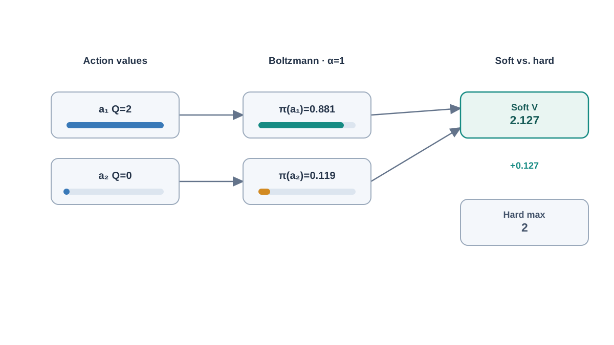
Take a state with two actions and $Q(s, a_1) = 2$, $Q(s, a_2) = 0$. Set $\alpha = 1$.

The soft value is:

$$V^*(s) = 1 \cdot \log\big(e^{2} + e^{0}\big) = \log(7.389 + 1) = \log(8.389) \approx 2.127$$

The Boltzmann policy is:

$$\pi^*(a_1 \mid s) = \frac{e^{2}}{e^{2} + e^{0}} \approx 0.881, \qquad \pi^*(a_2 \mid s) \approx 0.119$$

The hard-max value is $\max(2, 0) = 2$. The soft value is higher — $2.127$ — because the entropy term rewards keeping the second action alive. Now shrink the temperature to $\alpha = 0.1$:

$$V^*(s) = 0.1 \log\big(e^{20} + e^{0}\big) \approx 0.1 \cdot 20 = 2.0$$

The gap closes. The policy concentrates: $\pi^*(a_1 \mid s) \approx 0.9999$. As $\alpha \to 0$, the soft equations recover the standard Bellman equations, and the Boltzmann policy recovers the greedy argmax.

Reading the Temperature as a Mathematical Object

The temperature scales the entropy term relative to reward. It sets the exchange rate between expected reward and policy stochasticity. Two limits define its behavior:

• $\alpha \to 0$: the Boltzmann policy concentrates on the argmax, and the soft equations recover the standard Bellman equations.
• $\alpha \to \infty$: the policy flattens toward uniform, and reward stops mattering.

The temperature is also the dual variable of a constrained problem. Maximize reward subject to an entropy floor, and the Lagrangian produces the same objective with a temperature determined by the constraint. That is why automatic temperature tuning is a dual ascent step — you are solving for the multiplier that satisfies the constraint, not guessing a hyperparameter.

Note: The temperature is not a learning rate. It changes the optimum, not the step size toward the optimum. A learning rate controls how fast you move; the temperature controls where you are moving to.

The failure modes are symmetric. A fixed temperature that is too high makes the optimal policy deliberately suboptimal in reward terms — it will leave reward on the table to stay stochastic. A temperature that is too low reintroduces the deterministic collapse the entropy term was meant to prevent.

When Stochasticity Is Rewarded, Not Just Used

Exploration stochasticity is a means to gather data. It vanishes at convergence. Optimality stochasticity is part of the objective. It persists at convergence.

The soft optimal policy is stochastic even when the environment is deterministic and the reward is deterministic, because the entropy term is inside the return. This is the practical payoff of the derivation: the stochasticity is not a training artifact you anneal away. It is the answer.

When this is genuinely useful:

• Multi-modal action distributions where several actions are near-equally good, and committing to one mode is arbitrary.
• Robustness to perturbation, where a policy that spreads probability across near-optimal actions degrades more gracefully.
• Settings where a deterministic policy would overcommit to one mode before the critic has resolved the others.

When it is the wrong tool:

• Tasks with a single correct action where any deviation is costly. The entropy term will trade reward for diversity you do not want.
• Fixed temperature without regard to reward scale. A temperature tuned for one reward scale is wrong for another.

	Standard Bellman	Soft Bellman
Backup operator	$\max_a Q(s, a)$	$\alpha \log \sum_a \exp(Q(s, a)/\alpha)$
Optimal policy	Deterministic argmax	Boltzmann distribution
Value definition	$V = \mathbb{E}_\pi[Q]$	$V = \mathbb{E}_\pi[Q] - \alpha \mathbb{E}_\pi[\log \pi]$
Temperature role	None	Exchange rate between reward and entropy

From the Derivation to the Algorithm

The soft Bellman backup is the target the critic regresses toward. That is why entropy-regularized critics use a log-policy term in the target rather than a plain reward plus discounted value. The Boltzmann policy from the optimality derivation is the form the actor is pushed toward, which is why entropy-regularized actors are stochastic by construction.

I will stop at the equations here. The learning loop that turns these into an algorithm, and the continuous-control experiment that exercises them, are separate steps.

To verify the derivation against output rather than trusting it, implement the two-action example in a few lines:

import numpy as np

Q = np.array([2.0, 0.0])
alpha = 1.0

V_soft = alpha * np.log(np.sum(np.exp(Q / alpha)))
pi_soft = np.exp(Q / alpha) / np.sum(np.exp(Q / alpha))
V_hard = np.max(Q)

print(f"soft V: {V_soft:.4f}, hard V: {V_hard:.4f}")
print(f"policy: {pi_soft}")

Run it. Change alpha to 0.1 and watch the soft value converge to the hard value and the policy concentrate. The numbers should match the hand calculation above. If they do not, the derivation or the code has a bug — and finding which one is the point.

The test for whether stochasticity belongs in your objective is simple: does it survive at convergence? If it vanishes, it was exploration. If it persists, it was part of the return. Run the soft backup numerically against the standard one on a small problem, and let the gap between them tell you which regime you are in.