
Soft Actor-Critic Explained: Entropy-Regularized Learning for Continuous Control
Most actor-critic methods force you to choose between sample efficiency and stable exploration. Soft Actor-Critic (SAC) refuses the trade—and that refusal…

Key topics
Most actor-critic methods force you to choose between sample efficiency and stable exploration. Soft Actor-Critic (SAC) refuses the trade—and that refusal is not a trick. It is a redesign of the objective itself.
If you have worked with actor-critic methods, you already know the shape of the problem: the actor proposes actions, the critic scores them, and the gradient flows back to improve the proposal. SAC keeps that skeleton but changes what the critic is scoring and what the actor is optimizing for. The result is an off-policy algorithm that learns from stale experience, explores without collapsing to a greedy policy too early, and has become a default choice for continuous control.
The common mistake is to read SAC as "DDPG plus a stochastic policy." That framing misses the load-bearing part. The entropy term is not a bonus bolted onto the objective—it is what makes SAC's particular balance of exploration and exploitation work.
What SAC Actually Changes in the Actor-Critic Loop
Standard actor-critic maximizes expected return. Maximum-entropy RL adds a second term: the policy's entropy, weighted by a temperature coefficient. The objective becomes expected return plus expected entropy. In plain language: SAC wants a policy that gets high reward and keeps its options open.
That sounds like a minor modification. It is not. The entropy term changes what the critic estimates and what the actor optimizes. Instead of chasing the single best action, the policy is rewarded for maintaining a spread of good actions. That spread is what keeps exploration alive as learning progresses.
SAC learns three objects: two Q-critics and one stochastic policy. The original paper also trained a separate state-value network, but modern implementations fold that value estimate into the Q-functions. You can think of the architecture as two critics sharing one actor.
The soft Bellman target captures the shift in plain causal language. The value of taking an action in a state is no longer just the reward plus the discounted value of what comes next. It is the reward plus the discounted value of the next state plus a preference for actions the policy still supports. That preference term—the temperature times the negative log-probability of the sampled next action—is the entropy regularization showing up inside the value estimate itself.
If you have the actor-critic and maximum-entropy mental models in place, this section is your anchor. If not, treat it as the frame you will return to when the update loop gets dense.
Knowledge check
Check your understanding
Answer this question before you continue.
Why Two Critics and a Target Network
A single Q-network has a systematic flaw: it overestimates value. When you take a maximum over noisy estimates, the noise biases the result upward. In discrete action spaces, you can correct this by enumerating all actions and taking the true max. In continuous control, you cannot—the action space is dense, and there is no tractable way to search it exhaustively.
SAC's answer is clipped double-Q. Train two critics independently. When forming the target, take the minimum of their predictions. The minimum trims the optimistic bias because both networks would have to overestimate the same action for the bias to survive.
The two critics are not redundant. They are not averaging for accuracy. They are a bias-correction device, and treating them as a cheap ensemble is the wrong mental model.
Target networks add a second layer of stabilization. SAC does not hard-copy the critic weights into the targets periodically, the way DQN does. Instead, it uses Polyak averaging: after each update, the target networks move a small fraction of the way toward the current networks. This soft update keeps the target from jumping around, which matters because the critic is chasing a moving target that depends on its own predictions.
The deeper reason this machinery matters: in continuous action spaces, the policy must supply the next action for the target. There is no max-over-actions shortcut. The critic's target depends on what the actor proposes, which means the two networks are coupled in a way that discrete Q-learning never experiences. The double-Q and target smoothing are what keep that coupling stable.
Knowledge check
Check your understanding
Answer this question before you continue.
The Stochastic Policy and the Reparameterization Trick
SAC's actor is a squashed Gaussian. The policy network outputs a mean and standard deviation for each action dimension, and actions are sampled from that distribution. The "squash" is a tanh applied to the sampled value, bounding actions to a finite range like [-1, 1].
The stochasticity is not decorative. Entropy requires randomness, and a Gaussian gives a tunable amount of it per state. When the policy is confident, it narrows the distribution. When it is uncertain, it widens it. The entropy term in the objective is what prevents the distribution from collapsing to a near-deterministic point too early.
The reparameterization trick is what makes this trainable. Instead of sampling directly from the policy distribution—an operation with no gradient—you sample noise from a fixed distribution and push it through a deterministic function of the state. The action becomes a deterministic transformation of the state and noise, which means gradients can flow from the critic's score back through the action into the policy network.
The policy loss, in plain terms, pushes the actor toward actions the minimum critic values highly while resisting collapse to a single deterministic action. The entropy term acts as a spreading force. The critic acts as a focusing force. The balance between them is controlled by the temperature.
This is the piece that trips up readers coming from discrete-action RL. In discrete spaces, you can enumerate actions and compute their probabilities exactly. In continuous spaces, the policy must propose actions, and the gradient must flow through the proposal mechanism. The reparameterization trick is the bridge that makes that possible.
Knowledge check
Check your understanding
Answer this question before you continue.
Walking the SAC Update Loop
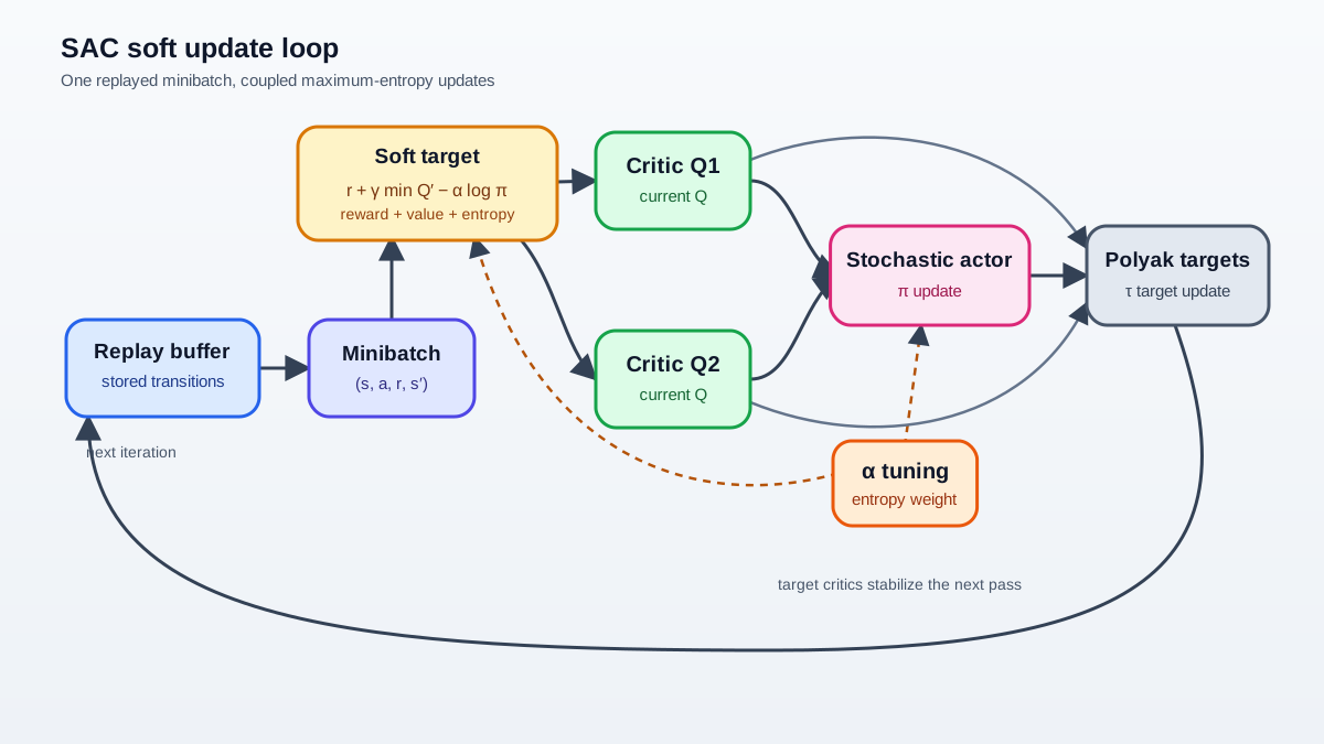
The SAC learning loop is best understood as a numbered pipeline. Each iteration follows the same sequence:
Step 1: Sample a minibatch. Pull transitions—state, action, reward, next state, done flag—from the replay buffer. The buffer holds experience collected across many versions of the policy, which is what makes SAC off-policy.
Step 2: Form the soft target. For each transition, sample a next action from the current policy at the next state. Compute the target as the reward plus the discounted minimum of the two target critics' predictions at that next state-action pair, plus the entropy contribution: the temperature times the negative log-probability of the sampled next action.
Step 3: Update the critics. Each critic is trained toward that target with a mean-squared Bellman error loss. The two critics get the same target but different predictions, which is what lets the minimum act as a bias correction.
Step 4: Update the policy. Sample actions from the current policy at the states in the minibatch, using the reparameterization trick. Push the policy toward actions the minimum critic values highly while keeping entropy high.
Step 5: Update the temperature. Adjust alpha to keep the policy's entropy near a target value.
Step 6: Polyak-average the targets. Move the target networks a small fraction toward the current critics.
A single flow diagram captures this: replay buffer to minibatch, then three loss paths—two critic losses and one policy loss—plus the temperature update and the target-network smoothing. The loop is compact, but every piece is doing a specific job.
Knowledge check
Check your understanding
Answer this question before you continue.
Automatic Temperature Tuning: What Alpha Is Really Doing
Alpha is the dial between expected return and policy entropy. A fixed alpha forces you to guess the right reward scale. If rewards are large, a fixed alpha becomes negligible and the entropy term stops mattering. If rewards are small, the entropy term dominates and the policy never learns to exploit.
Automatic tuning reframes the problem. Instead of choosing alpha, you choose a target entropy—a desired level of policy randomness—and let alpha adapt to hold the policy near it. The default target is typically the negative of the action dimension. A two-dimensional action space gets a target entropy of -2. The logic: each action dimension contributes roughly one unit of entropy, and the target scales with the space the policy must explore.
Alpha's behavior during training is a diagnostic signal. If alpha keeps climbing, the policy is being pushed to stay broad. That can mean the reward signal is weak, the task is genuinely hard to exploit, or something is wrong with how rewards are scaled. If alpha collapses to near zero, the entropy term has stopped mattering and the policy is free to become deterministic.
My rule: trust automatic tuning when you are exploring a new task and do not know the reward scale. Use a fixed alpha when you have a specific exploration-exploitation balance in mind and want to remove a variable from the experiment. Automatic tuning is not always better—it is one more learned quantity that can misbehave.
Where SAC Shines and Where It Breaks
SAC's strengths come from its design. Off-policy replay gives sample efficiency. Clipped double-Q and target smoothing give stability. The stochastic policy gives exploration that does not decay to greedy behavior too early.
The failure modes are equally specific.
The Gaussian policy is unimodal. SAC's actor can only represent one mode of action preference per state. If the optimal behavior is genuinely multimodal—two very different actions are equally good—the Gaussian will average between them and produce something mediocre. This is a structural limitation of the policy class, not a tuning problem.
Reward scale sensitivity returns without automatic tuning. If you fix alpha and the reward scale changes, you have effectively changed the entropy weight. The same alpha that worked for one task can be wrong for another.
The entropy objective can keep the policy too broad. In tasks where a near-deterministic final policy is required, the entropy term fights against precision. SAC may learn a policy that is still exploring when you need it to commit.
The decision boundary against alternatives is practical. Use SAC for continuous control when sample efficiency matters, you can tolerate a stochastic final policy, and old transitions remain useful for the current objective. Consider TD3 when you want a deterministic policy with similar off-policy efficiency. Reach for on-policy methods like PPO when you cannot trust the replay-buffer assumption—for example, when the environment dynamics shift or the reward structure makes stale experience actively misleading.
| SAC | TD3 | PPO | |
|---|---|---|---|
| Sample efficiency | High (off-policy) | High (off-policy) | Low (on-policy) |
| Final policy | Stochastic | Deterministic | Stochastic |
| Exploration mechanism | Entropy-regularized | Target policy smoothing | Policy gradient noise |
| Key stability device | Clipped double-Q + entropy | Clipped double-Q + delayed updates | Trust region / clipping |
Reading SAC's Training Curves Like a Builder
A healthy SAC run has a recognizable signature. Critic losses trend downward without diverging. Alpha settles near a stable value rather than climbing or collapsing. Policy entropy drifts toward the target instead of pinning at it or falling off a cliff.
The red flags are specific—but treat them as hypotheses, not verdicts. Alpha exploding upward can mean the entropy term is fighting a weak reward signal, or it can mean the reward scale is miscalibrated relative to your target entropy. Q-values diverging from actual returns means the critics are learning a fantasy. Policy entropy pinned at the target while returns stagnate can mean the policy is exploring forever without converting that exploration into improvement—or it can mean your log-probability computation is wrong.
When a run fails, my first question is not "which hyperparameter should I change?" It is "which of the three losses is misbehaving?" The critic losses, the policy loss, and the temperature loss each carry different information. Identify the broken signal before touching the knobs.
The practical next step is an experiment you can run today. Take a simple continuous-control benchmark, implement or import SAC, and log four quantities: alpha, policy entropy, both critic losses, and return. Then perturb one element—reward scale, target entropy, or replay buffer size—and watch which failure signal appears first. That single experiment will teach you more about SAC's mechanism than reading another explanation.
The mental model becomes durable when you can predict which component breaks under which pressure. Build the loop. Log the signals. Break one thing. Watch what moves.
Knowledge check
Final check
Finish the article by checking the ideas you just learned.
References
Research updated Sep 9, 2026


