
Continuous-Action Policies in Reinforcement Learning: Distributions, Bounds, and Noise
You move from discrete actions to continuous control, wire up a Gaussian policy head, and the agent either jitters uselessly around a target or slams…

Key topics
You move from discrete actions to continuous control, wire up a Gaussian policy head, and the agent either jitters uselessly around a target or slams itself into the action boundary. The network is fine. The problem is the unexamined assumptions about what the distribution's scale, support, and noise are actually doing to the learning loop.
Why Continuous Actions Break the Discrete Playbook
A discrete policy ends in a categorical head: a probability vector over a finite menu of actions. The network's job is to decide how much mass to put on each option. That mental model survives exactly until your action space becomes a real-valued vector.
Continuous-action policy reinforcement learning replaces "pick an action" with three design decisions the discrete case never forced you to make:
- Which distribution family the policy outputs.
- Whether that distribution's support matches the action bounds.
- How wide the distribution is at any given state.
The prerequisite mental model still holds: a parameterized policy maps observations to action probabilities. Continuous control just changes what "probability" means. Instead of mass spread over discrete options, you have a density over a continuous range, and sampling from that density produces the action.
The recurring failure is treating the Gaussian head as a drop-in replacement for the categorical head. It is not. A categorical distribution has natural boundaries built into its support. A Gaussian has none, and the moment your environment imposes limits, you inherit a problem the discrete playbook never had to solve.
Knowledge check
Check your understanding
Answer this question before you continue.
The Diagonal Gaussian Policy: Mean, Log-Std, and the Scale Question
The standard continuous policy head is a diagonal Gaussian. The network emits two vectors per action dimension: a mean, which represents the intended action, and a log-standard-deviation, which controls how much noise to add around that mean.
The log-std is the parameter beginners skip and later regret ignoring. It is learned, not fixed, because the agent must tune its own exploration as it gains confidence. Early in training, a wide distribution helps the agent discover which actions lead to reward. Later, the same distribution must narrow so the agent can execute precise control. The network has to learn that schedule itself, and the log-std is the lever it pulls.
Think of the scale as the exploration dial. The mean says "I think this is the right action." The standard deviation says "how sure am I?" A wide dial produces energetic exploration and imprecise execution. A narrow dial produces precise execution and no discovery.
The classic failure mode is the log-std drifting to extremes. Push it too negative and the policy freezes into near-deterministic actions, killing exploration before the value estimates have stabilized. Push it too positive and the agent produces pure noise, never converting what it learns into usable control. Both failures look like a broken network. Both are actually a scale parameter that nothing kept in check.
Knowledge check
Check your understanding
Answer this question before you continue.
The Bounds Problem: What Happens When Actions Must Stay in Range
Most continuous-control environments constrain actions to a finite interval. Torques, velocities, and joint angles all live inside physical limits, and benchmark environments typically normalize those limits to something like [-1, 1]. An unbounded Gaussian sampled naively will produce actions outside that range.
The bandage is clipping: sample from the Gaussian, clamp the result to the interval, and move on. It works well enough to get training running, and badly enough to quietly corrupt it.
Clipping concentrates probability mass at the boundary. When the mean sits near the edge of the action range, a large fraction of samples fall outside the valid interval and get clamped to the same boundary value. The effective distribution is no longer Gaussian. It is a Gaussian with a pile of probability mass stacked at the boundary, and the policy gradient assumes the sampled action came from the distribution the policy thinks it is using. That assumption is now false.
The boundary-effect bias is not a numerical nuisance. It distorts the gradient near the limits of the action range, which is exactly where a policy that wants to push a joint to its limit must learn clean signal. The agent learns a distorted map of its own action space.
Knowledge check
Check your understanding
Answer this question before you continue.
Squashing: Tanh and the Bounded Gaussian
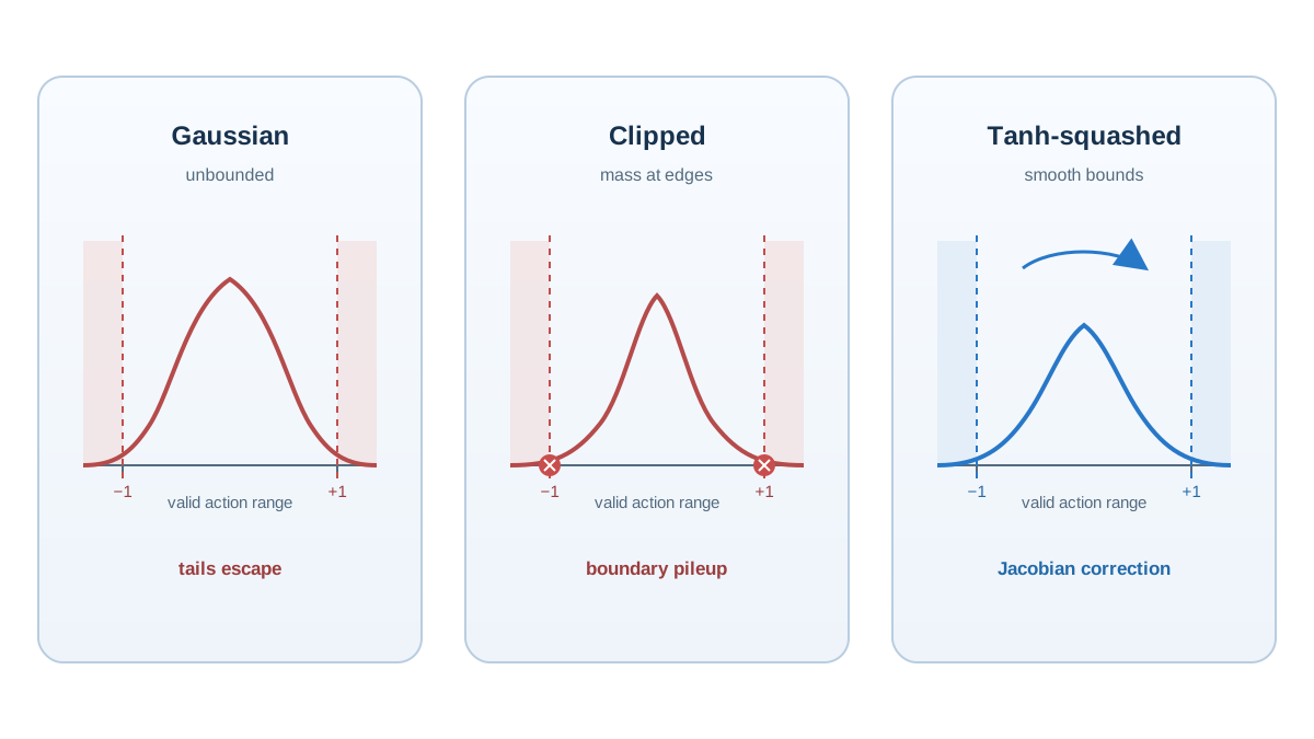
The cleaner solution is squashing. Sample from an unbounded Gaussian, push the result through a tanh function, and the output lands inside [-1, 1] by construction. No clamping, no mass piling at the boundary.
The cost is mathematical. Squashing changes the density. The log-probability used in policy-gradient updates must include a Jacobian correction for the change of variables. This is the term that makes tanh-squashed policies slightly more annoying to implement, and it is non-negotiable: skip the correction and the gradient is wrong.
Why squashing beats clipping comes down to smoothness. Tanh is differentiable across the entire action range, so the policy gradient flows cleanly even when the mean sits near the boundary. The distribution's mass redistributes smoothly toward the edges rather than stacking into a spike.
There is a tradeoff worth knowing. Tanh squeezes the tails of the Gaussian, which means extreme actions become exponentially unlikely. For most control tasks this is harmless, even desirable: the policy rarely needs to command a joint to its absolute limit with high precision. But if your task genuinely requires frequent extreme actions, the tanh-squashed Gaussian will fight you.
Finite-Support Alternatives: Beta and Beyond
Squashing solves the boundary problem by transforming an unbounded distribution. A different approach is to choose a distribution whose support natively matches the action bounds, eliminating the need for transformation entirely.
The Beta distribution lives on [0, 1] by construction. No squashing step, no clipping, no boundary bias. Research on continuous control has shown that finite-support distributions can reduce the estimation bias that clipping and squashing introduce near action limits, particularly in environments where the optimal policy spends significant time at the boundaries.
The tradeoff is practical. Beta distributions are less standard in RL frameworks, numerically trickier to sample and evaluate, and the log-probability computation is more involved than a Gaussian's. You are trading implementation convenience for cleaner boundary behavior.
My decision rule: start with a tanh-squashed Gaussian for standard benchmarks. It is the default for good reason. Reach for a finite-support family when boundary behavior is the dominant failure mode, when your policy needs to hold actions at their limits for extended periods, or when you have diagnosed that boundary bias is actively distorting learning.
Knowledge check
Check your understanding
Answer this question before you continue.
Stochasticity vs. Usable Control: Reading the Noise
The scale parameter is not just a detail of the distribution. It is the entire exploration strategy, and getting it wrong produces recognizable symptoms.
If the agent jitters around a target, never settling into precise control, the distribution is too wide. The mean has learned the right action, but the noise is drowning it out. If the agent never discovers better actions and converges to a mediocre solution early, the distribution collapsed too quickly. The log-std narrowed before the value estimates had enough signal.
There is a distinction worth keeping straight. A stochastic policy samples from a distribution for exploration. A deterministic policy with added noise, the DDPG/TD3 family, uses a separate mechanism: the actor outputs a deterministic action and exploration noise is added during training. These are different designs, not variations of the same thing. The stochastic policy's noise is baked into the gradient; the deterministic actor's noise is a training-time addition that gets stripped away at deployment.
That last point matters for evaluation. When you test a stochastic policy, use the mean action, not a sample. The noise exists to drive learning. At deployment, sampling from the distribution adds jitter that the policy did not learn to compensate for.
One practical warning before you train anything: normalize the action space to a symmetric range like [-1, 1]. Most algorithms assume a Gaussian initially centered at zero with unit standard deviation. If your environment uses [0, 1] or [-0.5, 0.5], the distribution's default scale fights the environment from the first step, and you will spend hours debugging what looks like a learning failure but is actually a scale mismatch.
Choosing a Policy Head for Your Problem
The decision framework is compact:
| Distribution | Native support | Boundary handling | Typical use case |
|---|---|---|---|
| Plain Gaussian | Unbounded | None needed | Genuinely unbounded actions |
| Clipped Gaussian | Unbounded | Clamping, biased | Quick experiments only |
| Tanh-squashed Gaussian | [-1, 1] | Smooth, differentiable | Standard continuous-control benchmarks |
| Beta / finite-support | [0, 1] or scaled | Built-in | Boundary-dominant tasks |
Use a tanh-squashed Gaussian for most standard continuous-control problems. Use a finite-support distribution when boundary bias is the dominant failure mode. Use a plain Gaussian only when actions are genuinely unbounded, which is rarer than you might think.
Do not reach for a stochastic distribution at all when you need deterministic control. Deterministic actor-critic methods trade away sampling noise for other exploration mechanisms, and they are the right tool when the policy's job is precise, repeatable action selection rather than exploration through stochasticity.
The unifying rule: the policy head is not an implementation detail. It encodes your assumptions about what actions are possible and how much the agent should explore. Get those assumptions wrong and no amount of tuning elsewhere will fix it.
The Experiment That Makes It Concrete
Pick a small continuous-control environment. Inspect the action bounds. Then deliberately test three policy heads on the same problem: an unbounded Gaussian, a clipped Gaussian, and a tanh-squashed Gaussian. Watch what happens at the boundaries. Watch when the noise collapses and when it never narrows.
The failure modes will not be subtle. The unbounded Gaussian will produce invalid actions. The clipped one will learn a distorted policy near the limits. The tanh-squashed one will behave, and you will finally see why the distribution family, its support, and its scale are the real architecture of continuous-action reinforcement learning.
Knowledge check
Final check
Finish the article by checking the ideas you just learned.
References
Research updated Sep 9, 2026


