Deterministic Policy Gradients Explained: Learning Continuous Actions Without Sampling a Distribution

A stochastic policy averages over actions. A deterministic policy climbs the critic's slope at the single action it outputs. That swap—from averaging to climbing—is the deterministic policy gradient idea, and it changes where your gradient comes from, how you explore, and what data you can use.

The Problem a Deterministic Actor Solves

In continuous control, your action space is a vector of real numbers: torques, joint angles, throttle settings. When you build a stochastic policy over that space, you fit a probability distribution—usually a Gaussian—and your policy gradient must account for every action the distribution could produce.

That is the crux. In a high-dimensional action space, you cannot enumerate all possible actions. You estimate the expectation by sampling from the policy's distribution, and each sample adds variance to your gradient. The more dimensions you control, the more samples you need to pin the gradient down.

A deterministic policy removes the action-distribution average from the update. Instead of outputting a distribution and sampling from it, the actor outputs one action per state: μ_θ(s). No distribution over actions, no sampling from it, no action-space integral in the gradient expression.

Notice what remains: the gradient still contains an expectation over states, usually estimated from samples collected by a behavior policy or drawn from a replay buffer. Determinism removes the action expectation, not all expectations and not all sampling. A stochastic policy estimates its action-distribution average through samples too—it never literally evaluates every continuous action.

This is the deterministic policy gradient theorem in its practical form: the actor updates its parameters by following the gradient of the critic's action-value estimate with respect to the action it outputs. If you already understand actor-critic methods, the architecture is familiar—a critic estimates Q, an actor adjusts the policy—but the relationship between them changes. In a stochastic actor-critic, the actor follows a probability-weighted average over actions. In a deterministic actor-critic, the actor climbs the slope of Q at the exact action it chose.

How the Actor Update Actually Works

The deterministic actor update is a chain rule, and keeping the two links straight is the difference between understanding the method and just running it.

The actor wants to maximize Q^μ(s, μ_θ(s))—the critic's estimate of how good it is to take the actor's action in state s. To update the actor's parameters θ, you need the gradient of that value with respect to θ. The chain rule splits it into two factors:

∇_θJ(θ) = E[∇_aQ(s, a)|_a=μ(s) · ∇_θμ_θ(s)]

The first factor asks: if the action moved slightly, how would the critic's estimate change? That is the slope of the action-value surface with respect to the action. The second factor asks: if the policy parameters moved slightly, how would the output action change? That is the standard backpropagation path through the actor network.

Here is the subtle part that trips up most people on first contact: the critic's parameters are treated as constants during the actor update. You are not backpropagating through the critic's loss. You are using the critic as a fixed landscape, asking which direction in action space increases its value, then asking which direction in parameter space produces that action change. Two separate gradient computations, chained together.

Because the policy is deterministic, the actor only needs Q(s, μ(s))—one evaluation at the action the policy actually produces. Contrast that with the stochastic actor-critic update, where the gradient is an expectation over actions drawn from π_θ(a|s), weighted by the policy's own probabilities. The stochastic version spends its compute averaging; the deterministic version spends its compute climbing.

Why Deterministic Policies Need Off-Policy Learning

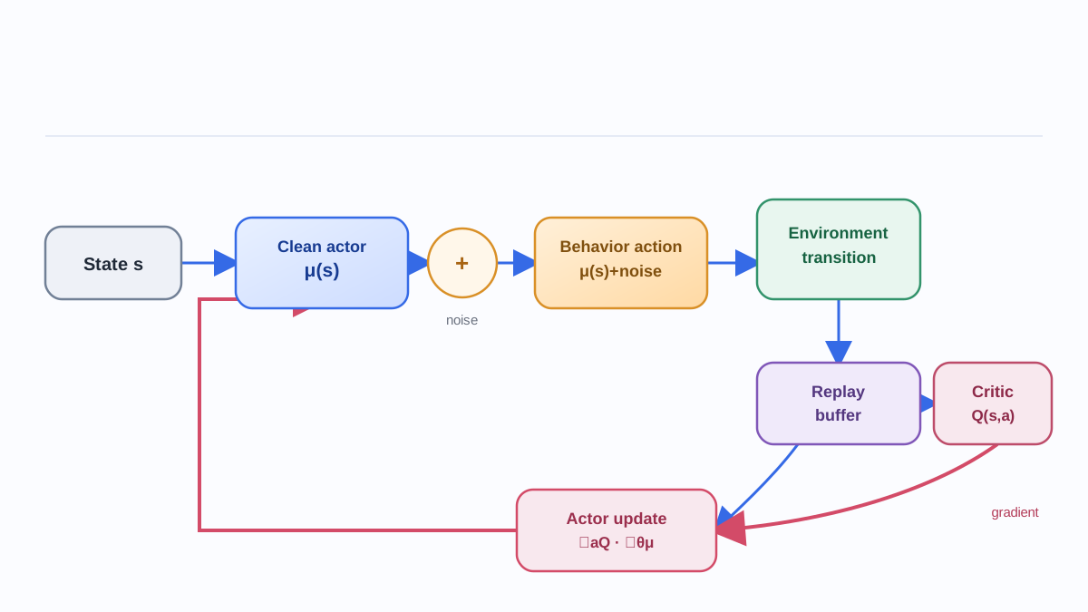
Here is the tension that defines the entire family: a deterministic policy cannot explore on its own.

Think about what exploration means in a stochastic policy. The policy itself assigns probability mass to multiple actions. Even a near-greedy policy samples actions you have not tried before, and those samples are exactly what the gradient needs to improve. The policy's own randomness is its exploration mechanism.

A deterministic policy has no such mechanism. In a given state, it always outputs the same action. If you tried to learn on-policy with a deterministic actor, you would only ever see the actions the actor already believes are best. You would never discover whether a slightly different action was better, because you would never take it.

The solution is to decouple the behavior that collects data from the policy being learned. You explore with a stochastic behavior policy—one that adds noise, jitters around, tries alternatives—while you learn a deterministic target policy from the data that behavior policy collects. This is an off-policy actor-critic, and it is the design that makes deterministic policy gradients work in practice.

This is also why deterministic policy gradient methods pair naturally with a replay buffer. Since the data comes from a behavior policy that differs from the target policy, you need a way to reuse and learn from off-policy transitions. The replay buffer stores them, and the actor and critic update from sampled batches.

There is a second benefit worth naming precisely. In a stochastic off-policy setting, you normally need importance sampling to correct for the mismatch between the behavior policy and the target policy. The deterministic policy gradient removes the integral over actions, which means that correction term disappears from the actor update. The gradient remains approximately valid off-policy because you are no longer averaging over an action distribution that differs between behavior and target.

Exploration: The Price of Determinism

The tradeoff is now visible, and it is worth stating plainly: a deterministic actor trades away its own exploration for a cheaper, more direct gradient. The price is paid in injected noise.

In practice, that means adding noise to the action at training time. The standard approach is Gaussian noise added to the actor's output—the behavior policy becomes μ_θ(s) + noise, while the target policy remains the clean deterministic μ_θ(s). At test time, the noise is removed entirely. Exploration is a training-time device, not part of the learned policy.

This creates a sharp contrast with the maximum-entropy and soft actor-critic family. In those methods, exploration is inside the objective: the policy is rewarded for keeping probability mass spread across actions, so diversity is part of what the policy optimizes. A deterministic actor has no such internal pressure. Its exploration budget is whatever noise you inject, and if that noise is poorly tuned, the policy either fails to cover the action space or wanders too far from good actions to learn anything stable.

The data-efficiency picture follows from this. A deterministic actor can be more sample-efficient per gradient step in high-dimensional action spaces, because it is not spending samples on averaging over actions it will never take. But that efficiency is conditional on the injected noise actually covering the regions the critic needs to evaluate accurately. If the noise is too small, the critic never learns about promising alternative actions. If it is too large, the data is mostly noise and the critic's estimates are unreliable.

When a Deterministic Actor Is the Right Tool

The decision boundary is not about which method is newer or more popular. It is about the structure of the task and the quality of the critic you can train.

Deterministic actors are attractive when the action space is high-dimensional and a single decisive action per state is natural. Think robotic control: given the current joint positions and velocities, one torque vector is usually the right commitment. In that regime, the deterministic gradient's efficiency is a real advantage, because the stochastic alternative spends samples exploring actions that a competent policy would never seriously consider.

But action dimension is a pressure, not a guarantee. The deeper question is whether a near-greedy action is appropriate and whether your critic can be trained accurately around exploratory data. Deterministic actors struggle when the optimal policy is genuinely multimodal or when the environment rewards action diversity. If multiple very different actions lead to similar returns, a deterministic actor must pick one and stick with it. A stochastic or entropy-regularized policy can keep options open, maintain coverage, and adapt when the situation changes.

The practical failure mode is worth internalizing: a deterministic actor is only as good as the critic's slope it climbs. If the critic is inaccurate in unexplored regions—and it will be, because the actor only visits actions the noise allows—the actor chases a misleading gradient. This is why target networks and delayed updates matter so much in modern implementations. They are not hyperparameter niceties; they are the stabilizers that keep the actor from running off the edge of a critic that has not learned the terrain yet.

My rule of thumb: use a deterministic actor when the task demands a decisive continuous action and you can afford the off-policy machinery. If the task rewards keeping options open, or if your critic is hard to make accurate, a stochastic or entropy-regularized policy is the safer bet.

The Mental Model That Keeps It Straight

Here is the image to hold onto. A stochastic policy is a surveyor: it takes many measurements across the action space, averages them, and moves in the direction of the weighted consensus. A deterministic policy is a climber: it puts one hand on the slope at its current position and pulls itself upward.

The surveyor is robust but slow—every measurement costs samples. The climber is fast but blind—it only knows the slope where it stands, and if the map (the critic) is wrong, it climbs the wrong hill.

The analogy has a boundary. The surveyor does not literally measure every point on a continuous action surface; it estimates its average from samples. And the climber's speed advantage only matters when the map is accurate enough to trust. What the image captures correctly is the source of gradient information: stochasticity supplies an action distribution inside the policy objective, while determinism relies on behavior noise and local critic derivatives.

The exploration burden moves from inside the policy to outside it. That single shift explains the architecture: the off-policy learning, the replay buffer, the injected noise, the target networks. Every design choice in the deterministic policy gradient family is a response to the fact that the policy itself cannot explore.

If you want to make this concrete, run a small continuous-control experiment. Take a pendulum or simple robotic arm environment, train a deterministic actor, and vary the injected noise. Hold the environment, update budget, and evaluation policy fixed. Then watch three things: return versus environment steps, the diversity of actions stored in the replay buffer, and evaluation performance with noise removed. Too little noise and the policy converges to a narrow behavior that never discovers better actions; too much and the critic never stabilizes. The experiment will teach you more about the exploration tradeoff than any amount of reading.

From there, the natural continuation is DDPG itself—the algorithm that made deterministic policy gradients work with deep networks—and its successor TD3, which fixes the overestimation bias that plagues naive deterministic critics. The mental model you have now is the foundation both algorithms build on.

References

Research updated Sep 9, 2026