Maximum-Entropy Reinforcement Learning: Why Good Policies Keep Options Open

Most reinforcement learning tutorials treat randomness as a ladder: you need it to explore, and once training converges, you kick it away. Maximum-entropy reinforcement learning makes a stranger claim. Sometimes the stochastic policy is not a compromise. It is the answer.

The Misconception: Randomness Is Only a Training Crutch

Standard RL maximizes expected return. Mathematically, that objective is satisfied by any policy that achieves the maximum—so the optimizer has no reason to prefer diversity. The result is a well-known drift: policies collapse toward deterministic behavior, because a greedy policy and a stochastic policy with equal expected return score identically, but the greedy one is simpler to find.

Beginners internalize this as a law of nature. You add noise for exploration, anneal it away, and the trained agent should be a clean, deterministic controller. That story is true for a large class of algorithms. It is not true for maximum-entropy RL.

The reframe is subtle and worth sitting with: in maximum-entropy reinforcement learning, diversity is not a means to an end. It is a term in the objective itself. The policy is rewarded for keeping options open. Acting randomly is not tolerated despite the reward—it is part of what "good" means.

That raises the question this article answers: when is acting slightly randomly genuinely the right answer, and when is it a tax on performance?

What Entropy Measures in a Policy

Before the objective, you need a precise handle on the entropy term. Policy entropy is not a loose synonym for randomness. It is a measure of how evenly probability mass is spread across actions at a given state.

A deterministic policy has zero entropy at that state: all mass sits on one action. A uniform policy over three actions has maximum entropy: the mass is spread as evenly as possible. The Shannon entropy formula, H(π(·|s)) = −E[log π(a|s)], is just a way of counting how surprised you are on average by samples from the policy. Concentrated distribution, low surprise, low entropy. Spread distribution, high surprise, high entropy.

Two details matter for the mental model.

First, entropy is computed per state, then summed over the trajectory. The objective does not care that your policy is diverse "overall." It cares about diversity at every decision point. A policy that is random in easy states and deterministic in hard ones can have high total entropy, but the objective rewards exactly the opposite: it wants you to keep options open precisely where the future is uncertain.

Second, the entropy term is not a property of the actions themselves. It is a property of the distribution. A coin flip has one entropy. A coin flip you have weighted 90/10 has less. The same two actions can produce very different entropy values depending on how the policy spreads its bets.

A small discrete example makes this concrete. Suppose a state has three actions. A policy that assigns probabilities (1, 0, 0) has entropy 0. A policy that assigns (1/3, 1/3, 1/3) has entropy log(3), the maximum for three actions. A policy at (0.8, 0.1, 0.1) sits between them. The entropy term is a continuous dial on how committed the policy is at that state—not a binary random/not-random switch.

The Objective: Reward Plus a Diversity Bonus

The maximum-entropy objective modifies the standard expected-return objective by adding an entropy bonus at every timestep:

J(π) = E[Σ r(s_t, a_t) + α H(π(·|s_t))]

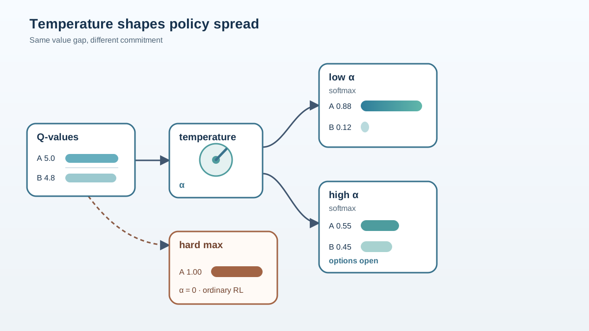
The temperature coefficient α is the dial between two masters. High α tells the policy that diversity is worth more; the policy spreads probability mass even at the cost of reward. Low α tells the policy that reward dominates; the entropy term becomes a weak nudge rather than a real constraint. At α = 0, you have ordinary RL.

The interesting consequence is the form of the optimal policy. In standard RL, the optimal policy at a state is the argmax over Q-values: pick the best action, ignore the rest. In maximum-entropy RL, the optimal policy takes a Boltzmann form:

π*(a|s) ∝ exp(Q*_soft(s, a) / α)

Action probability is proportional to the exponential of the soft Q-value divided by the temperature. This is where the "soft" naming comes from in soft Q-learning and soft actor-critic. The hard max over actions becomes a softmax over Q-values. Actions with near-tied Q-values share probability mass. Actions with clearly higher Q-values dominate—but never absolutely, unless α is driven to zero.

Picture the Q-value landscape at a state. Standard RL draws a vertical line at the argmax: one action gets everything. Maximum-entropy RL smooths that line into a softmax curve. If two actions are genuinely close in value, the policy hedges. If one action is clearly superior, the softmax concentrates on it. The temperature controls how sharp that concentration is.

Why Keeping Options Open Helps: The Robustness Argument

The standard justification for stochastic policies is exploration: noise helps you find reward. Maximum-entropy RL offers a deeper reason, and confusing the two leads to a weak mental model.

A policy that injects its own noise is, in effect, practicing recovery from disturbances. When the policy acts randomly, it lands in states it did not plan for, and it learns to act well from those states. If the environment dynamics shift later, the change looks like just another disturbance the policy has already trained on. Standard RL trains a policy to execute one clean path. Maximum-entropy RL trains a policy that has seen—and recovered from—its own messes.

This intuition has a formal backbone. Maximum-entropy RL maximizes a lower bound on a robust RL objective: a policy with high entropy-regularized reward is guaranteed to achieve decent reward even when an adversary chooses the dynamics to make the policy look bad. The entropy bonus is not a heuristic that happens to help. It is a principled hedge against distribution shift.

The "many paths to the goal" image captures the behavioral difference. If several routes solve a task, standard RL commits to one—usually the shortest—and becomes brittle if that route is blocked. Maximum-entropy RL tries all of them, prefers shorter paths proportionally, and retains the ability to switch when the world changes. The benefit is not just finding reward. It is retaining behavioral flexibility that pays off exactly when the training distribution stops matching the deployment distribution.

The Soft Bellman View: Where the Mechanism Lives

If you know actor-critic methods, you already have the architecture. The new piece is what the critic is optimizing for.

In standard RL, the Bellman backup takes a hard max over next actions: the value of a state is the reward plus the value of the best next action. Entropy regularization changes this. The entropy bonus flows into the value function, and the hard max becomes a soft max:

Q_soft(s, a) = r(s, a) + γ E[V_soft(s')]

where V_soft(s') = α log Σ exp(Q_soft(s', a') / α)

The soft max is a smooth approximation of the hard max. It is always at least as large as the hard max, and it approaches the hard max as α shrinks. But it has a crucial property: it does not produce a sharp cliff between the best action and the second-best action. Near-tied actions produce near-tied values, and the value landscape becomes smooth instead of jagged.

This smoothness is not cosmetic. It changes what the critic learns and how the actor updates. In soft actor-critic (SAC), the critic learns soft Q-values, and the actor is trained to match the softmax policy implied by those values. The result is an off-policy maximum-entropy actor-critic: the critic estimates the entropy-regularized value, and the actor is pulled toward the Boltzmann policy rather than the argmax.

The practical consequence is a learning signal that is gentler and more informative. Standard Q-learning can oscillate violently when two actions have near-equal values, because a tiny change in estimates flips the argmax. The soft Bellman backup absorbs that instability. The policy does not need to commit until the evidence is clear.

When the Entropy Bonus Hurts

Maximum-entropy RL is not universally beneficial, and pretending otherwise leads to failed experiments.

The failure mode is precise: when the optimal policy genuinely requires low-entropy action selection, the entropy bonus flattens the Q-landscape peak and dilutes focus in narrow feasible regions. Imagine a task where only a precise action succeeds—a narrow gap, an exact insertion, a finely timed maneuver. The entropy bonus actively pushes probability mass away from the narrow winning region toward actions that cannot succeed. Forced diversity becomes a tax on achievable reward.

The temperature coefficient is the lever, and it is a sensitive one. Too high, and the policy never commits: it stays diffuse even where the Q-landscape has a clear winner. Too low, and the regularization is meaningless: the policy collapses to near-deterministic behavior and you have paid the complexity cost of maximum-entropy RL without receiving its benefits.

The practical response is adaptive temperature tuning. Entropy-constrained SAC treats the entropy target as a constraint rather than a fixed bonus, adjusting α during training to maintain a desired level of stochasticity. This works well in practice, but it does not solve a deeper limitation: action entropy alone does not guarantee high state entropy. If many actions lead to the same next state—action redundancy—a policy can have high action entropy while visiting very few states. The diversity that matters for exploration is diversity of experience, not diversity of action labels.

Use maximum-entropy RL when tasks have many near-equivalent solutions, noisy dynamics, or a need for robustness under distribution shift. Be cautious when the task demands precision and the feasible region is narrow. The same objective that makes a policy gracefully hedge can make it frustratingly indecisive.

Reading a MaxEnt Policy: What to Look For

A healthy maximum-entropy policy has a recognizable signature: it keeps meaningful spread across actions that are genuinely near-tied in value, and it concentrates on the clear winner when one exists. The spread is not uniform noise. It tracks the Q-landscape.

The failure signature is equally recognizable. A policy that stays diffuse even where the Q-landscape has a sharp peak is telling you the temperature is too high. The policy is not exploring—it is refusing to decide. Conversely, a policy that collapses to determinism everywhere is telling you the entropy term has stopped mattering.

One practical detail reveals how sensitive this dial is: implementations that automatically tune α typically optimize its logarithm, not the value itself. The temperature spans orders of magnitude across tasks, and optimizing in log space keeps updates stable. When you see this in code, read it as a warning—the coefficient is fragile enough that direct optimization causes problems.

The mental model closes here. The entropy term is not decoration on the reward. It changes what the value function means, which changes what the policy commits to. A maximum-entropy policy is not a noisy version of a deterministic policy. It is a different kind of decision-maker: one that treats keeping options open as part of the job.

The Decision Rule

Treat the entropy bonus as a modeling choice about what kind of behavior counts as good—not a training trick to be switched on and off. If you believe the task has many acceptable solutions and the world might shift under you, maximum-entropy RL is not a compromise. It is the correct objective. If you believe the task demands one precise action and the environment is stable, the entropy bonus is a tax.

The way to make this concrete is to run it. Take a small continuous-control task and compare a maximum-entropy agent against a plain actor-critic at different temperature settings. Watch where the MaxEnt policy stays diffuse—those are the states where the agent believes multiple actions are near-equivalent. Watch where it commits—those are the states where one action clearly dominates. Then change the dynamics slightly and see which policy survives the shift.

That experiment will teach you more than any derivation. The entropy term is a claim about the world: that diversity has value beyond the immediate reward. Whether that claim is true is not a theoretical question. It is an empirical one, and now you know exactly what to look for.

References

Research updated Sep 9, 2026