Generalized Advantage Estimation Explained: A Bias-Variance Dial for Actor-Critic RL

Every actor-critic user hits the same wall shortly after their first working implementation: the advantage estimate looks fine in theory, but the policy update behaves erratically, and the usual fixes pull in opposite directions. Trust the value function too much and the gradient chases its errors. Trust the sampled rewards too long and the gradient drowns in noise. Generalized advantage estimation exists because this tension is not a bug to eliminate—it is a dial to turn.

The Advantage Estimation Problem an Actor-Critic Can't Avoid

The policy gradient needs a direction to push the policy: raise the probability of actions that worked better than expected, lower the rest. The advantage function, A(s, a) = Q(s, a) − V(s), provides exactly that signal. The critic's value function makes the estimate tractable by serving as a baseline, but the critic is never perfect during training. That imperfection is where the real design problem begins.

You have two naive ways to estimate the advantage from a collected trajectory, and both are broken in instructive ways.

The one-step TD advantage uses a single reward followed by a bootstrap:

Â_t^(1) = r_t + γV(s_{t+1}) − V(s_t)

This estimate has low variance because it only sums one stochastic reward. But it leans entirely on the critic's prediction for the next state. When the value function is wrong—and early in training it always is—that error flows directly into the advantage and biases the policy update.

The full Monte Carlo advantage sums every reward to the end of the episode before subtracting the baseline:

Â_t^(∞) = r_t + γr_{t+1} + γ²r_{t+2} + ... − V(s_t)

This estimate is unbiased in the ideal case: it uses real rewards, not critic predictions, so value-function error cannot bias it. But it sums many stochastic rewards, and variance grows with the horizon. In a long continuous-control episode, that noise can swamp the gradient signal entirely.

The core problem is that estimator error has two distinct sources. Bias comes from bootstrapping on an imperfect value function. Variance comes from accumulating stochastic rewards across time. Reduce one and you amplify the other.

The weak mental model here is treating lambda as a config constant to copy from someone else's working implementation. The strong mental model is seeing it as a dial that trades these two error sources against each other—and knowing which direction to turn it based on what your critic knows and how far your rewards look into the future.

From One-Step Residuals to a Weighted Sum Across Time

The building block of generalized advantage estimation is the TD residual:

δ_t = r_t + γV(s_{t+1}) − V(s_t)

This looks similar to the one-step advantage, but it plays a different role. A residual is a local surprise signal: how much better or worse did this single step go than the critic predicted? GAE's insight is that you can sum residuals forward in time to reconstruct longer-horizon advantage estimates.

Sum one residual and you get the one-step advantage. Sum two:

δ_t + γδ_{t+1} = r_t + γr_{t+1} + γ²V(s_{t+2}) − V(s_t)

That is the two-step advantage. Sum k residuals and you reconstruct the k-step advantage, which uses k real rewards before bootstrapping on the critic. Each additional residual you include extends the estimator's trust in real rewards by one more step.

GAE's move is to take a weighted average of all these n-step estimators, with weights decaying exponentially:

Â_t^GAE = (1 − λ) Σ_{k=0}^∞ (γλ)^k δ_{t+k}

The (1 − λ) factor is a normalizer. Without it, the weighted sum would grow with the horizon instead of staying on the same scale as a single advantage estimate. With it, the weights form a proper averaging scheme.

To see what this actually does, imagine a small trajectory where the critic makes a noticeable error at step t+2. The residual at that step, δ_{t+2}, will carry that error. A one-step estimator never sees it. A two-step estimator includes it once, unweighted. GAE includes it with weight (γλ)², so the error's influence on the advantage at step t is real but attenuated by distance. The further a residual sits from the current state, the less it matters—and lambda controls exactly how fast that influence fades.

Lambda as the Bias-Variance Dial

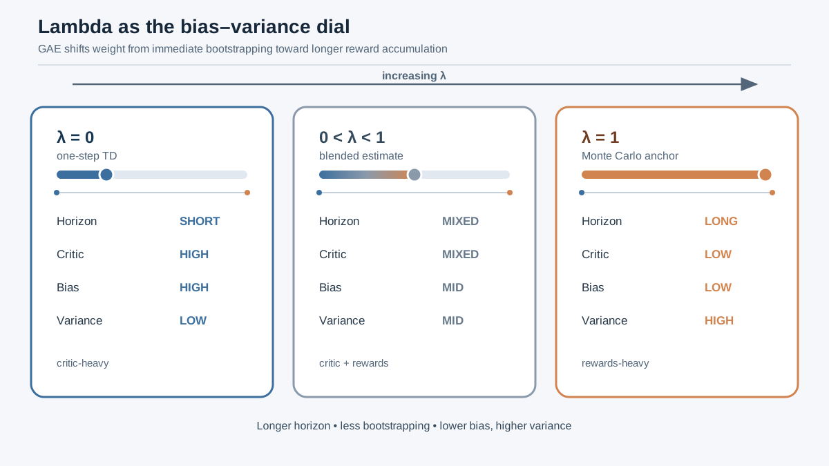
Lambda's boundary cases are worth internalizing because they anchor everything between them.

At λ = 0, the sum collapses to a single term. GAE becomes the one-step TD advantage. The estimator trusts the critic immediately, uses almost no real reward information beyond the current step, and inherits the critic's bias directly. Variance is at its minimum.

At λ = 1, the geometric sum expands fully. GAE becomes the Monte Carlo advantage, using every reward to the episode's end. In the ideal full-trajectory case, bootstrapping bias disappears entirely, but variance grows with the horizon, and in long episodes it can become unmanageable. In practical truncated-rollout implementations, a bootstrap boundary can still remain at the cutoff, so treat this boundary as the conceptual anchor rather than an absolute guarantee about every implementation.

Intermediate values interpolate between these extremes. Higher lambda means the estimator trusts real rewards longer before leaning on the critic's bootstrap, trading lower bias for higher variance. Lower lambda means the estimator cuts off reward noise sooner and leans on the critic earlier, trading variance for bias.

A subtle point deserves emphasis: gamma and lambda both discount, but they do different jobs. Gamma shapes the return definition itself—how much future rewards matter to the objective. Lambda shapes how much the estimator leans on the critic versus observed rewards. Gamma is part of the problem you are solving. Lambda is part of the estimator you built to solve it.

This distinction explains a practical observation: good lambda values are typically lower than gamma. Practitioners rarely push lambda to 1, because doing so reintroduces the Monte Carlo variance that actor-critic methods were designed to avoid. Lambda is not a knob on the return. It is a knob on how much you trust your critic versus your own sampled rewards.

Why GAE Is Computed Backward Through the Trajectory

The weighted-sum form is useful for understanding, but implementations rarely compute it directly. Instead, they use a recursive form that falls out of the geometry of the sum:

Â_t = δ_t + γλÂ_{t+1}

This recursion makes the computation a single backward pass through the trajectory. Start at the last step, compute its advantage, then walk backward, each step adding its own residual to a discounted, decaying memory of all future residuals.

The recursion works because each advantage carries the accumulated tail of everything behind it. When you compute Â_{t+1}, it already contains δ_{t+1} plus γλ times Â_{t+2}, and so on. Multiplying by γλ as you move backward applies the exponential decay automatically, so one pass produces the same result as the explicit weighted sum.

This structure should feel familiar if you have seen eligibility traces. GAE is the advantage-space analogue of a trace that fades across time: a decaying memory that connects the present decision to future consequences. The connection is structural, not identical—GAE operates on advantage estimates, not on policy-parameter credit—but the fading-memory shape is the same.

The backward sweep has a practical consequence that catches many implementers: episode boundaries must zero out the recursion. If an episode ends at step t, the advantage at t+1 belongs to a different episode, or to nothing at all. Without masking the recursion at done flags, the estimate leaks across episode resets, contaminating the first few advantages of the next trajectory with rewards from the previous one.

Reading Lambda's Effect on Update Behavior

Lambda changes more than the estimator's statistical properties. It changes what the policy gradient actually does during training.

With low lambda, updates react to short-horizon deviations from the value function's prediction. The policy chases immediate surprises: a reward that arrived when the critic expected none, or failed to arrive when the critic expected one. This makes the policy responsive to dense feedback, but it also makes it sensitive to critic error, because the critic's mistakes at nearby states dominate the estimate.

With high lambda, updates integrate longer-horizon reward information. The policy can respond to delayed consequences: a sequence of actions whose payoff only appears several steps later. But the gradient carries more noise per batch, because each advantage sums more stochastic rewards.

The practical failure modes follow directly. Lambda too low can make the policy myopic, overfitting to the critic's local errors instead of learning genuine long-term consequences. Lambda too high can make updates unstable in long-horizon continuous-control tasks, where the accumulated variance overwhelms the signal.

Choosing a value means weighing several factors at once, and no single monotonic schedule follows from the mechanism alone:

• Critic quality. A poor critic injects error into every residual. Lower lambda limits how far that error propagates forward, but it also makes the estimate lean harder on the same flawed critic at the next state. Critic quality alone does not tell you which direction to turn.
• Reward delay. When the consequences of an action appear many steps later, higher lambda preserves that delayed signal by carrying residuals forward. But it pays for that reach with added variance.
• Rollout horizon. Truncated rollouts leave a bootstrap boundary at the cutoff. Very high lambda can amplify whatever error the value function has at that boundary.
• Update stability. If gradient steps are already noisy, the added variance from high lambda can make training unstable regardless of the other factors.

This is why GAE is the default advantage estimator in PPO and TRPO pipelines for continuous control. Locomotion tasks like the MuJoCo environments have dense reward structure but long horizons, and the bias-variance spectrum matters at every stage of training.

If you want to develop a feel for this, run a small lambda sweep on a continuous-control task. Hold rollout length, gamma, batch size, and the random seed protocol fixed, then compare candidate values. Watch the right signals:

• Estimator dispersion. Measure the variance or spread of the advantage estimates within a batch before any normalization. Higher lambda should widen the distribution; lower lambda should tighten it.
• Sign consistency. Run repeated rollouts with the same policy and check whether the sign of each advantage stays stable. Frequent sign flips across runs indicate noise dominating the estimate.
• Critic behavior. Track the TD residuals or value loss. If residuals stay large, the critic is still poor, and no lambda setting will remove that error from the estimate.
• Return stability. Compare the smoothed policy return across several seeds. The right lambda is the one where the policy improves steadily without either symptom dominating.

One caution: raw advantage magnitude is diagnostic context, not a target. Many implementations normalize advantages before the policy update, which changes the scale you observe. Do not tune toward smaller numbers; tune toward the setting where the estimator's dispersion, sign consistency, and resulting return curves tell a coherent story.

When GAE Is the Right Tool and When It Isn't

GAE is the right default for on-policy actor-critic methods—PPO, TRPO, A2C—that collect trajectory batches and need one advantage estimate per transition. The estimator's design matches the data these algorithms collect: full trajectories from the current policy, with a critic that can be evaluated at every state.

It is less central in off-policy methods. Algorithms that replay past transitions or use different advantage formulations face a different design question, and GAE's trajectory-based structure does not transfer cleanly.

GAE also does not fix a bad value function. It only tunes how much the estimator trusts one. A poorly trained critic biases every lambda setting, because its errors leak into the residuals that GAE sums. Improving the critic is always the higher-leverage intervention.

It does not solve exploration or credit assignment across very long horizons by itself. GAE is an estimator, not a learning algorithm. It shapes how the gradient sees the data it already collected; it does not decide which data to collect or resolve the structural credit-assignment problem across hundreds of steps.

When the horizon is short, the bias-variance spectrum collapses. With only a few steps per episode, the Monte Carlo advantage has little room to accumulate variance, and the one-step advantage has little room to accumulate bias. GAE's tuning range matters less, and a simpler estimator often suffices.

The boundary with eligibility traces is worth stating precisely. Both use a fading-memory shape to interpolate across time, but they operate on different objects. Eligibility traces assign credit to policy parameters across recently visited states and actions. GAE estimates advantages by blending TD residuals. The shared geometry is real; the mechanism is not identical.

The practical takeaway is to treat lambda as a dial you turn deliberately, not a constant you copy. Ask two questions before setting it: How good is my critic right now? How far in the future do the consequences of my actions appear? The answers tell you which direction to turn. Then run a controlled sweep, watch the estimator's dispersion and update stability shift, and let the observed behavior confirm what the mechanism predicts.

References

Research updated Sep 9, 2026