Value Decomposition in Multi-Agent RL: Learning Team Actions From Local Views

A team shares one reward, but at execution time each agent must pick its own action from only its own observation. Value decomposition answers that specific constraint: learn a joint value function that can be torn apart into local pieces without breaking the team optimum.

The Problem a Joint Value Function Can't Solve Alone

In cooperative multi-agent reinforcement learning, the cleanest theoretical object is a centralized joint action-value function Q_tot(s, a) over the global state and the joint action space. In principle, this function captures everything the team needs: given the full state and every agent's action, it predicts the team's expected return.

In practice, that function is unusable at execution time. No agent sees the full state. No agent observes the other agents' actions before choosing its own. Each agent operates on its own partial observation history, and by the time the joint action is assembled, the decision has already been made.

This is the execution constraint that defines the entire value decomposition branch of multi-agent RL: each agent must select argmax over its own action given only its local observation history. If you train a centralized Q_tot and then try to extract decentralized policies from it, you face an immediate question: how does any individual agent know which of its actions contributed to the joint optimum?

Centralized training with decentralized execution (CTDE) solves the information problem—agents can share state, actions, and rewards during training. But CTDE alone doesn't solve the action-selection problem. Knowing the joint value function exists doesn't tell you how to decompose it into per-agent decision rules.

That's the design question at the heart of value decomposition multi agent reinforcement learning: how do you train a joint value function whose argmax can be recovered by independent local argmax operations? The answer is to build the factorization into the architecture from the start, rather than trying to reverse-engineer it after training.

The IGM Principle: When Local Greedy Choices Match the Team Optimum

The Individual-Global-Max (IGM) principle is the formal anchor criterion that organizes this entire field. It states that the joint argmax of Q_tot equals the tuple of individual argmaxes of the per-agent Q_i functions:

argmax_a Q_tot(s, a) = (argmax_{a_1} Q_1(τ_1, a_1), ..., argmax_{a_N} Q_N(τ_N, a_N))

Read that equation carefully. It says something precise and something limited. The precise claim is about alignment: if each agent greedily picks the action that maximizes its own Q_i, the resulting joint action is exactly the one that maximizes the team's Q_tot. No coordination protocol needed. No negotiation at execution time. Each agent acts selfishly on its own value function, and the team lands on the joint optimum.

The limited claim is just as important. IGM guarantees alignment of argmaxes. It does not guarantee that the learned Q_i values are accurate estimates of individual contributions to the team outcome. An agent's Q_i might be a poor estimate of its actual marginal contribution, yet still produce the correct greedy action. Conversely, Q_i values can look reasonable while the joint argmax is wrong.

IGM is a consistency condition on the factorization, not a learning algorithm by itself. It tells you what property your architecture must satisfy, but it doesn't tell you how to learn the Q_i functions or how to structure the mixing mechanism. Every value decomposition method you encounter should be evaluated through this lens: does its factorization satisfy IGM, and what class of joint value functions can it represent while doing so?

VDN: The Sum That Started the Branch

Value Decomposition Networks (VDN) represent the simplest possible factorization: the joint value is the sum of per-agent utilities, each conditioned on that agent's local observation-action history.

Q_tot(s, a) = Σ_i Q_i(τ_i, a_i)

Training follows a straightforward recipe. Compute the summed Q_tot, calculate the joint TD loss against the team reward, and let gradients flow back through the sum to each agent's network. The sum operation is differentiable and transparent—each agent's network receives gradient signal proportional to how much its Q_i contributed to the joint prediction error.

The sum trivially satisfies IGM. The argmax of a sum of independent terms is the tuple of individual argmaxes, because each term depends on only one agent's action. If agent 1 changes its action, only Q_1 changes, so the joint argmax decomposes cleanly.

That triviality is both the strength and the ceiling. A pure sum cannot represent team interactions where the value of a joint action is not additive. Consider two agents whose combined effect is superadditive—the team succeeds only when both act in a coordinated way, and the value of that coordination exceeds the sum of individual contributions. Or subadditive—two agents doing the same task redundantly produce less value than the sum of their independent efforts. VDN's linear decomposition has no way to represent either effect.

The practical failure mode follows directly. VDN can underperform when coordination requires representing nonlinear team effects. In tasks where agents genuinely need to complement each other's actions, the additive assumption flattens the value landscape and the team learns a compromised policy.

QMIX: Adding a Mixing Network Without Breaking IGM

QMIX replaces the fixed sum with a learned mixing network that combines per-agent utilities into Q_tot. The mixing network takes the individual Q_i values as inputs and produces the joint value, conditioned on the global state.

The innovation is the constraint that makes this work. QMIX constrains the mixing network's weights to be non-negative, which enforces monotonicity: increasing any Q_i must increase Q_tot.

Why does monotonicity suffice for IGM? If Q_tot is monotone in each Q_i, then the joint argmax is reached by maximizing each Q_i independently. Raising any individual Q_i can only raise the joint value, never lower it, so the greedy local policy and the joint optimum align.

This is the QMIX intuition in one sentence: use a more expressive mixing function, but restrict it to functions where local improvement always means team improvement.

The tradeoff is the mirror image of VDN's limitation. Monotonicity buys decentralized execution but restricts the class of joint value functions QMIX can represent. It cannot capture joint actions where one agent's value increase should decrease the team value. If the optimal team strategy requires an agent to take a locally worse action so that another agent can succeed, QMIX's monotone mixing network cannot represent that relationship—it would need a negative weight to express the tradeoff.

Contrast this with VDN. QMIX is strictly more expressive: the sum is a special case of a monotone mixing function. But both are IGM-satisfying factorizations with different representational ceilings. VDN can only represent additive structure. QMIX can represent any structure where the joint value is monotone in each agent's local value.

What Decomposition Can and Cannot Represent

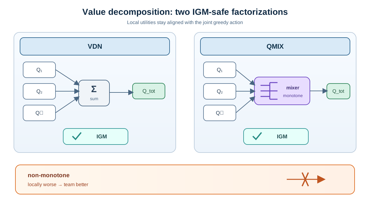
The representational boundary deserves to be explicit, because it determines when each method is the right tool.

Additive factorization captures independent contributions. It works when agents' effects on the team outcome are roughly separable—each agent's value doesn't depend much on what the others do. In that regime, VDN is simple, stable, and hard to beat.

Monotone factorization captures a wider class. QMIX can represent team effects where agents amplify or dampen each other's contributions, as long as the relationship stays monotone. If agent 1's success makes agent 2's actions more valuable, a positive mixing weight captures that amplification.

The boundary appears when the team optimum requires an agent to sacrifice its own local value. Picture a task where two agents must coordinate so that one takes a locally worse action to enable the team win. The optimal joint policy assigns agent 1 a low-value action because that action unlocks a much larger gain for agent 2. A monotone mixing network cannot represent this: expressing "agent 1's value should decrease so the team value increases" requires a negative weight, which violates the constraint.

This is the decision rule I use when choosing between decomposition methods: the question is not which algorithm is newer or more popular, but which representational class your task actually needs. Start with VDN when interactions are weak and simplicity matters. Move to QMIX when you observe team effects that look monotone—amplification, complementarity, coordination bonuses. Recognize when neither suffices, because your task's optimal policy genuinely requires an agent to act against its own local value.

Richer methods exist beyond these two, including approaches that relax the monotonicity constraint or use more general mixing structures. But the IGM lens is the right way to evaluate any of them. Ask what representational class the factorization permits, and whether that class can express your task's coordination structure.

Common Failure Modes When Decomposition Goes Wrong

Value decomposition fails in predictable ways, and each failure traces back to a specific mechanism.

Reward sparsity. Decomposition methods need sufficiently dense team rewards to learn meaningful per-agent utilities. With sparse rewards, the credit signal never reaches individual agents—the joint TD error arrives rarely, and when it does, the gradient through the mixing structure is too diffuse to shape each Q_i. The result looks like no learning at all: agents drift, and the team never discovers coordinated behavior.

Non-stationarity from teammates. If other agents' policies shift during training, each Q_i is chasing a moving target. Agent 1's optimal action depends on what agent 2 is doing, and agent 2 is learning too. The mixing network must absorb that drift, but it can only do so if the training signal is strong enough to distinguish "agent 2 changed its policy" from "agent 1's value estimate is wrong."

Observation leakage at execution. If a Q_i was trained using information unavailable at execution time, the greedy local policy silently degrades. This is a deployment mismatch: the network learned to rely on a feature it can't access when actually making decisions. The training curves look fine because the information was present during learning; the evaluation fails because it's gone.

Overfitting the mixing network to the global state. The mixer can learn to compensate for weak per-agent utilities. If the global state is rich enough, the mixing network can essentially memorize the correct joint value while the local Q_i functions remain poor on their own. The team looks coordinated during training, but the individual agents have learned nothing useful—they're puppets whose strings are pulled by the mixer.

Each failure is diagnosable by the same test: inspect whether local greedy actions stay aligned with the joint optimum during evaluation. If you freeze the Q_i functions and let each agent act greedily on its own observation, does the team still achieve the coordinated behavior you saw during training? If not, the decomposition is doing the work, not the agents.

Choosing a Decomposition for Your Problem

Value decomposition is the right tool when you have a cooperative task with a shared team reward, a CTDE setup, and a genuine need for decentralized execution at deployment. That last condition matters more than people expect. If a centralized controller can act at runtime—if you have the state, the communication bandwidth, and the latency budget—you don't need decomposition at all. Train a joint Q-function and use it directly.

Value decomposition is the wrong tool in three situations. Competitive or mixed settings where agents have opposing objectives break the shared-reward assumption entirely. Tasks where the team optimum genuinely requires an agent to act against its own local value exceed the monotone representational class. And settings where decentralized execution isn't actually required make the whole framework unnecessary complexity.

My practical guidance is to start with VDN as a baseline. It's simple, stable, and gives you a reference point for how much coordination your task actually requires. If VDN performs well, your task may not need complex factorization. If it struggles and you can see team interactions in the reward structure, move to QMIX. And when you evaluate any factorization you encounter, apply the IGM test: does local greedy action selection reproduce the joint optimum under your specific reward and observation structure?

The choice between decomposition methods is about the representational class your task needs, not about which algorithm is newer. VDN and QMIX are both IGM-satisfying factorizations with different ceilings. Your job is to know which ceiling your task requires—and to recognize when the answer is neither.

References

Research updated Sep 9, 2026