
Credit Assignment in Multi-Agent RL: Which Agent Caused the Outcome?
Your team just won. The shared reward arrives, positive and unambiguous. Every agent updates its policy as if the victory were its own doing—and that is…

Key topics
Your team just won. The shared reward arrives, positive and unambiguous. Every agent updates its policy as if the victory were its own doing—and that is precisely the problem.
In multi-agent reinforcement learning, a team outcome is a single scalar produced by a joint action. No agent can see its own marginal contribution hiding inside that number. This is the collective credit assignment problem: turning one shared reward into per-agent learning pressure when the contributions that produced it are deeply entangled.
Why a Shared Reward Leaves Every Agent Guessing
Single-agent RL already wrestles with temporal credit assignment—connecting a late reward back to the action that caused it. Multi-agent credit assignment stacks a second attribution problem on top: the reward is not just delayed in time; it is shared across agents who acted together. You now have to answer when the right thing happened and which agent did it.
The formal setting makes the difficulty precise. In a Decentralized Partially Observable Markov Decision Process (Dec-POMDP), agents share one team reward function but act on local observations. The reward depends on the joint action—the combined choices of every agent—not on any individual action. When two agents must both pull levers to open a door, the reward arrives only after both have acted. Agent A cannot tell whether its pull mattered, whether Agent B's pull mattered, or whether both were necessary. The scalar contains no per-agent information.
The naive approach—treating the shared reward as if it were each agent's individual reward—looks harmless on paper. Each agent runs its usual policy update, receives the team reward, and adjusts. But the update quietly assumes something false: that every agent caused the entire outcome. The joint action space grows exponentially with the number of agents, and the reward is a function of that entire space. No single agent's marginal effect is visible in the scalar. Every agent's gradient gets the full team signal, as if each one had acted alone.
Knowledge check
Check your understanding
Answer this question before you continue.
The Two Failure Modes of Naive Credit
When you ignore the attribution problem, two distinct failure modes emerge. They look like opposites, but they share a root cause: the shared scalar does not contain per-agent information.
Credit hijacking happens when an agent that contributed nothing useful still receives the full team reward. Imagine a warehouse robot that spends its shift circling aimlessly while its teammate stacks every pallet. The team gets the completion bonus, and the circling robot's policy is reinforced for circling. Its irrelevant actions get credit they never earned. The more agents on the team, the easier it is for any single agent to free-ride on the collective outcome.
Credit starvation is the mirror image. A genuinely critical agent—the one whose action was necessary for success—sees its contribution lost in the noise of many teammates' updates. The signal that should have been loud arrives as a whisper, and its policy barely changes.
These are not tuning problems. You cannot fix them with a larger learning rate or more exploration. The shared scalar is structurally incapable of telling any agent whether its specific action mattered. And the problem compounds with the non-stationarity of multi-agent settings: as teammates update their policies, the answer to "who deserves credit" shifts underneath you. Attribution is a moving target because the contributors keep changing.
Note: A shared reward is not literally divided into equal portions. Every agent may receive the same scalar. The real problem is that the scalar cannot distinguish a pivotal action from a redundant one or an irrelevant one—so the learning signal each agent extracts is ambiguous, not merely diluted.
Knowledge check
Check your understanding
Answer this question before you continue.
Counterfactual Reasoning: What Would Have Happened Without You?
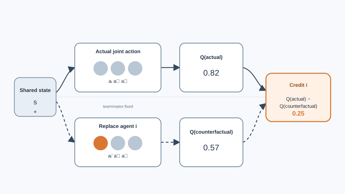
One family of solutions asks a direct question: what would the team outcome have been if this agent had acted differently? The difference between the actual outcome and that counterfactual baseline is the agent's credit.
This is the intuition behind Counterfactual Multi-Agent Policy Gradients (COMA), the canonical example of explicit credit assignment. COMA uses a centralized critic to estimate the counterfactual advantage of each agent's action. For each agent, it compares the team's Q-value under the actual joint action against the Q-value under the same joint action but with that agent's action replaced by a baseline. The gap between those two values is the agent's marginal contribution.
The mechanism is clean, but it carries real costs. The counterfactual baseline requires a centralized critic that can evaluate the joint state-action space, and it demands repeated value estimates for every agent at every step. Sample cost climbs. Complexity climbs. And there is a subtler limitation worth naming honestly: the baseline is derived from the current joint action, not the optimal one. Credit can point toward locally better behavior while missing globally superior alternatives. The counterfactual tells you what changed relative to where you are, not relative to where you should be.
Picture the same joint state branching into two paths: the actual action sequence and the counterfactual one. The centralized critic evaluates both. The difference between the branches is the credit signal. It is a powerful idea—but it is expensive, and it can lead you toward local optima when the current joint policy is far from optimal.
Knowledge check
Check your understanding
Answer this question before you continue.
Value Decomposition: Splitting the Team Q-Value
The second major family takes a different route. Instead of asking what each agent did, it imposes a structure on the global value function that makes per-agent learning signals fall out naturally.
Value Decomposition Networks (VDN) make the simplest assumption: the global Q-value is the sum of individual agent Q-values. Each agent learns its own local value function, and the team's value is just the sum. This is computationally cheap and scales well, but the additive assumption is restrictive. It cannot represent tasks where agent contributions interact nonlinearly—where the value of two agents acting together is greater than the sum of their individual values.
QMIX relaxes this with a monotonic mixing network. The global Q-value becomes a nonlinear combination of per-agent values, with the constraint that improving an individual agent's local value always improves the global value. This preserves the individual-global-max property: each agent can greedily select the action that maximizes its local value, and the joint action will maximize the global value. The nonlinearity gives QMIX more expressive power than VDN while keeping decentralized execution practical.
It helps to separate three claims that often blur together. A decomposition method may (1) represent the team value as a function of local values, (2) select decentralized greedy actions that respect the global optimum, and (3) provide an interpretable per-agent credit signal. VDN and QMIX deliver the first two. The third—explicit attribution—is not what they are built for. They are implicit credit assignment methods: they never name which agent caused what. Instead, they shape learning so each agent's local value function tracks its own contribution. The structural assumption does the attribution work silently.
That is both the strength and the weakness. Decomposition is sample-efficient and scales, but it imposes assumptions that can break when agent contributions are genuinely interdependent in ways the chosen structure cannot express.
| Approach | Mechanism | Cost | Choose When | Avoid When |
|---|---|---|---|---|
| Naive shared reward | Treat team reward as individual | Minimal | Weak coupling, dense rewards, homogeneous roles | Tight coordination, sparse rewards, heterogeneous roles |
| Counterfactual (COMA) | Compare actual vs. baseline outcome | High: centralized critic, repeated estimates | You can estimate individual action effects and need a sharp signal | Many agents with entangled effects; limited compute |
| Decomposition (VDN) | Global Q = sum of local Qs | Low | Contributions are roughly additive | Strong interaction effects between agents |
| Decomposition (QMIX) | Monotonic nonlinear mixing of local Qs | Moderate | Nonlinear value structure with decentralized execution | Non-monotonic tasks where a local improvement hurts the team |
Knowledge check
Check your understanding
Answer this question before you continue.
When Credit Assignment Gets Harder: Broken Assumptions
The clean two-family story—counterfactual versus decomposition—hides several assumptions that real tasks routinely violate. Each complication below breaks a specific assumption, and each has a distinct consequence for how you should think about attribution.
Subset rewards break the single-team assumption. Some rewards are earned by a subgroup, not the whole team. Two agents coordinate to capture a flag while three others hold a defensive line. A global decomposition misses which agents actually cooperated. The reward structure itself is not a single scalar to split; it is a collection of overlapping subgroup outcomes. For counterfactual methods, this means the baseline must be computed over the relevant subgroup, not the full team. For decomposition methods, it means a flat additive or monotonic split cannot represent which subset earned the reward.
Multi-level credit breaks the single-granularity assumption. Agents may cooperate at different granularities simultaneously: individual actions matter, but so do joint actions and correlated action patterns across larger groups. Standard methods assume one flat split. Recent work formalizes credit assignment levels—the number of agents cooperating to earn a reward—and builds advantage functions that reason across individual, joint, and correlated actions simultaneously. The practical consequence: if your task has rewards at multiple cooperation scales, neither a purely individual counterfactual nor a purely additive decomposition will capture the structure.
Asynchronous decisions break the synchronous timing assumption. Standard credit assignment assumes agents decide in lockstep: joint action at time t, shared reward at time t+1. Real systems have agents deciding and executing at different times. One agent commits to an action while another is still deliberating. The synchronous credit model has no clean way to attribute a reward to decisions made at different moments. Counterfactual methods struggle because the "joint action" is not well-defined when decisions are staggered. Decomposition methods struggle because the value function assumes a single decision point.
Offline data breaks the intervention assumption. When you only have logged data, you cannot run counterfactual rollouts. The counterfactual reasoning needs causal structure to identify which agents actually influenced the reward. Without the ability to intervene, attribution requires explicit causal models of the data-generating process.
These are open research boundaries, not solved problems. Each one marks an assumption that the basic methods quietly make—and that real tasks quietly violate.
Choosing a Credit Assignment Strategy
The practical question is not which method is best. It is which failure mode your task actually exhibits—and which assumptions you can afford to make.
Use naive shared reward when coordination is weak, rewards are dense, and agents have roughly homogeneous roles. If every agent faces similar situations and contributes in similar ways, the attribution error is tolerable. You are paying a small tax for simplicity. Do not use it when one agent's action can be decisive while others merely support—that is exactly the setting where credit starvation will quietly cripple learning.
Use value decomposition when you need decentralized execution at scale and the task's value structure fits the decomposition assumption. If per-agent local values give a useful learning signal, methods like QMIX give you scalability without a centralized critic at execution time. Do not use additive decomposition (VDN) when agent contributions interact strongly. Do not use monotonic decomposition (QMIX) when a task requires one agent to sacrifice its local value for the team—monotonicity forbids that tradeoff by construction.
Use counterfactual methods when you can estimate individual action effects and need a sharper per-agent signal. If one agent's decision is decisive and the rest are supporting cast, the counterfactual baseline gives you exactly the attribution that decomposition hides. Do not use them when many agents' effects are deeply entangled—the counterfactual for each agent becomes expensive to estimate and increasingly unreliable.
The honest boundary: no method removes the underlying ambiguity when agent contributions are genuinely entangled. Counterfactual methods trade cost for attribution sharpness. Decomposition methods trade expressiveness for sample efficiency. Neither can extract per-agent information from a scalar that never contained it. They can only impose structure that makes learning tractable despite the ambiguity.
This is an engineering tradeoff, not a correctness hierarchy. The right choice depends on your team size, your execution constraints, and which failure mode—credit hijacking or credit starvation—actually threatens your task.
The Diagnostic Habit
Rather than memorizing method names, build the habit of diagnosing your task's failure mode first. Here is a workflow that works in practice:
- Hold learned teammates fixed. Freeze the policies of all agents except one.
- Intervene on that agent. Run the episode with its actual action, then with a counterfactual action substituted in. Compare team return.
- Repeat across agents. You will quickly see which agents' actions move the team outcome and which do not.
- Inspect per-agent learning signals. Look at the advantages or local values each agent is receiving. Are irrelevant agents getting large positive updates? That is credit hijacking. Is a pivotal agent's signal indistinguishable from noise? That is credit starvation.
- Run an ablation. Remove one agent's contribution entirely and measure the team return drop. This tells you the agent's actual marginal value—and whether your chosen method's implicit attribution matches reality.
Name the failure mode, then pick the attribution strategy that targets it. The shared reward will never tell you which agent caused the outcome. Your job is to build a learning signal that does not pretend otherwise.
Knowledge check
Final check
Finish the article by checking the ideas you just learned.
References
- Nucleolus Credit Assignment for Effective Coalitions in Multi-agent Reinforcement Learning
- Multi-level Advantage Credit Assignment for Cooperative Multi-Agent Reinforcement Learning
- [2312.03644] MACCA: Offline Multi-agent Reinforcement Learning with Causal Credit Assignment
- [PDF] Learning Implicit Credit Assignment for Cooperative Multi-Agent ...
Research updated Sep 9, 2026


