
Test Value Factorization in a Small Multi-Agent Coordination Game
Two agents. Three actions each. Nine joint outcomes. If you cannot find the coordination failure in a table that small, you will not find it in a training…

Key topics
Two agents. Three actions each. Nine joint outcomes. If you cannot find the coordination failure in a table that small, you will not find it in a training curve that large.
This is a falsification drill. You are going to build the smallest machine that shows where decentralized greedy selection stops recovering the team-optimal joint action — and then you are going to edit the payoff table until the assumption visibly breaks. One file, standard library only, brute-force enumeration. No learning, no function approximation, no partial observability.
What This Exercise Assumes and What It Proves
I am assuming you already know centralized training with decentralized execution, and that you have met the individual-global-max consistency condition: the joint argmax over the centralized value function should equal the tuple of per-agent argmaxes over local utilities. If that sentence is doing heavy lifting for you, read the monotonicity derivation first and come back. Here I only need the claim, not the proof.
The claim under test: if local utilities are combined additively or monotonically, greedy per-agent action selection recovers the joint argmax.
That claim is a conditional. It holds when the factorization is exact. It fails when the task's payoff contains an interaction term the mixer cannot express. The counterexample target is a payoff table where the joint optimum requires at least one agent to accept a locally worse action.
Scope limit, stated up front so you do not over-generalize: this is a one-shot, fully observable, fully enumerable game. There is no learning loop, no neural network, no observation noise, no opponent. What you observe here is a property of the payoff structure and the mixing function. It says nothing about whether a given algorithm will converge on a real task.
Why brute force is the right tool: with two agents and three actions, enumeration is nine joint actions. Exhaustive search is faster, more trustworthy, and easier to debug than any optimizer you could point at this problem. When the search space is small enough to enumerate, enumerate.
The Game: Two Agents, Three Actions, One Payoff Table
Two agents, A and B. Each chooses from actions 0, 1, 2. The team value depends on the pair.
| A \ B | 0 | 1 | 2 |
|---|---|---|---|
| 0 | 4 | 0 | 0 |
| 1 | 0 | 1 | 0 |
| 2 | 0 | 0 | 8 |
Before you run anything, find the joint optimum by eye. Then find what each agent would pick if it only saw its own row or column. Hold both answers.
The interaction pattern encoded here is a coordination payoff: the high value of 8 appears only when both agents choose action 2. Every mismatched pair collapses to 0 or 1. This is the shape that additive and monotonic mixers struggle with, and the rest of the exercise makes that struggle printable.
One convention matters before we write code. Local utilities are each agent's own reward component, not the team value. If you define them as the team value split evenly, the greedy choice trivially matches the optimum and you will have proven nothing. The ambiguity between "per-agent reward component" and "counterfactual marginal" changes what "greedy" means, and I am picking the first definition because it is the one that produces the failure.
Knowledge check
Check your understanding
Answer this question before you continue.
Enumerate Joint Actions and Print the Optimum
Save this as factorization_probe.py. Standard library only.
import itertools

ACTIONS = [0, 1, 2]

# Joint payoff table: joint_value[(a, b)] = team value
JOINT = {
    (0, 0): 4, (0, 1): 0, (0, 2): 0,
    (1, 0): 0, (1, 1): 1, (1, 2): 0,
    (2, 0): 0, (2, 1): 0, (2, 2): 8,
}

def enumerate_joint():
    rows = [(ja, v) for ja, v in JOINT.items()]
    rows.sort(key=lambda r: (-r[1], r[0]))
    return rows

def joint_optimum(rows):
    return rows[0]

if __name__ == "__main__":
    rows = enumerate_joint()
    best_ja, best_v = joint_optimum(rows)
    print("Joint action ranking (value desc, action asc):")
    for ja, v in rows:
        print(f"  {ja} -> {v}")
    print(f"\nJoint optimum: {best_ja} with value {best_v}")
Expected output:
Joint action ranking (value desc, action asc):
  (2, 2) -> 8
  (0, 0) -> 4
  (1, 1) -> 1
  (0, 1) -> 0
  (0, 2) -> 0
  (1, 0) -> 0
  (1, 2) -> 0
  (2, 0) -> 0
  (2, 1) -> 0

Joint optimum: (2, 2) with value 8
The ranking matters more than the winner. Ties and near-ties are exactly where decentralized selection gets fragile, because a tie-break rule that happens to pick the optimum can hide a coordination problem that a different tie-break would expose. The code sorts by value descending, then by joint action ascending. That is arbitrary. Remember it, because it will matter in the failure-mode section.
Knowledge check
Check your understanding
Answer this question before you continue.
Compute Local Utilities and Greedy Choices
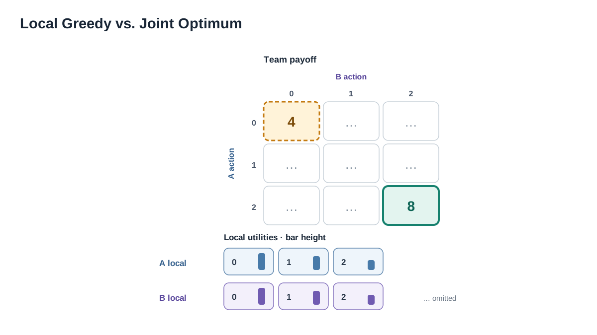
Now add the local utility table. Keep it separate from the joint table so you can see they are not the same object.
# Local utilities: agent's own reward component, independent of the other agent.
LOCAL_A = {0: 4, 1: 1, 2: 0}
LOCAL_B = {0: 4, 1: 1, 2: 0}

def greedy_action(local):
    # argmax with lowest-action tie-break
    return max(local.keys(), key=lambda a: (local[a], -a))

def locally_greedy_joint():
    return (greedy_action(LOCAL_A), greedy_action(LOCAL_B))

if __name__ == "__main__":
    # ... previous output ...
    ga = greedy_action(LOCAL_A)
    gb = greedy_action(LOCAL_B)
    greedy_ja = (ga, gb)
    greedy_value = JOINT[greedy_ja]
    print(f"\nAgent A greedy action: {ga} (utility {LOCAL_A[ga]})")
    print(f"Agent B greedy action: {gb} (utility {LOCAL_B[gb]})")
    print(f"Locally greedy joint action: {greedy_ja} -> team value {greedy_value}")
    print(f"Joint optimum:              {best_ja} -> team value {best_v}")
    print(f"Coordination cost:          {best_v - greedy_value}")
Expected output:
Agent A greedy action: 0 (utility 4)
Agent B greedy action: 0 (utility 4)
Locally greedy joint action: (0, 0) -> team value 4
Joint optimum:              (2, 2) -> team value 8
Coordination cost:          4
There it is. Two printed lines that disagree. Each agent maximizes its own utility by choosing action 0, and the resulting joint action is worth 4 — half the team optimum of 8.
The mechanism is plain causal: each agent is optimizing a projection of the team value onto its own action axis. That projection throws away the interaction term. Agent A's local utility for action 0 is 4, but that 4 only materializes if B also picks 0. A's utility for action 2 is 0, but that 0 becomes 8 if B also picks 2. The local utility cannot see the conditional. It sees a marginal, and the marginal is blind to the pair.
This is the IGM condition failing, shown as two printed lines rather than a proof. The joint argmax is (2, 2). The tuple of local argmaxes is (0, 0). They are not the same joint action, so no mixing function that preserves the local orderings can recover the optimum from these utilities.
Knowledge check
Check your understanding
Answer this question before you continue.
Why Additive and Monotonic Mixing Cannot Fix This Table
Additive case. If team value is a sum of local utilities, then Q_joint(a, b) = Q_A(a) + Q_B(b). The interaction term — the part of the joint value that depends on the pair and not on either agent alone — is identically zero. Any payoff that depends on the combination cannot be represented. Full stop.
Monotonic case. Monotonicity preserves the ordering of each agent's utilities under the mixer. It does not add expressiveness for interaction terms. A monotonic mixer can represent "higher local utility for A implies higher joint value, holding B fixed" — but it cannot represent a value that is high only for one specific combination and low for all others. Our (2, 2) -> 8 row is exactly that shape.
The arithmetic. Define the interaction term as joint value minus the sum of local utilities:
interaction = JOINT[(2, 2)] - (LOCAL_A[2] + LOCAL_B[2])
# 8 - (0 + 0) = 8
For the coordination row, the interaction term is 8. For (0, 0), it is 4 - (4 + 4) = -4. The interaction term is not small and not zero. It is the entire signal.
Be precise about what monotonicity does buy. It guarantees consistency between local and joint argmax when the factorization is exact. That is a guarantee about consistency, not about expressiveness. A monotonic mixer that cannot represent the interaction term will be consistent with a wrong joint value function. Consistency with the wrong function is not a win.
This is a representational limit of the mixing function, not a training failure. No amount of data fixes it. More episodes, more seeds, more gradient steps — none of them will teach an additive mixer to represent a term that is structurally outside its function class.
Modify the Table Until the Assumption Breaks
Now you become the experimenter. Three edits, each with a checkable outcome.
Edit 1 — make the coordination payoff strictly dominant. Change (0, 0) from 4 to 2. Re-run. The joint optimum is still (2, 2) at 8, but the locally greedy joint action is still (0, 0), now worth 2. The coordination cost jumps from 4 to 6. The failure is not a near-tie artifact; it gets worse as the interaction term grows.
Edit 2 — make the table additive by construction. Replace the joint table with JOINT[(a, b)] = LOCAL_A[a] + LOCAL_B[b] for every pair. Re-run. The locally greedy joint action now matches the joint optimum. This is the control case, and it proves the script is not broken. The assumption is doing real work. The failure in the original table is caused by the interaction term, not by a bug in the enumeration.
Edit 3 — introduce a tie in the joint table. Set (0, 1) and (1, 0) both to 4, matching (0, 0). Re-run. The printed ranking changes — three rows now share the value 4 — but the locally greedy choice does not move. The tie-break rule in enumerate_joint silently picks one of the tied rows as the "optimum," and if that row happens to be the greedy one, you will conclude decentralized selection succeeded when it merely got lucky. This is the trap the failure-mode section warns about.
Keep the modified table. It is a reusable counterexample. Any time you implement a new factorization method, drop this table in as a fixed test case and check whether the method recovers (2, 2) from the local utilities. If it cannot, you have found its representational boundary in about ten seconds of compute.
Knowledge check
Check your understanding
Answer this question before you continue.
Failure Modes and Debugging Signals
Mismatched indexing. If the joint table is keyed by action names and the local tables by action indices, you get a silent off-by-one that looks exactly like a real coordination failure. Print both keys before you trust the gap.
Local utilities defined as the team value split evenly. This makes the greedy choice trivially match the optimum and hides the entire point. If your coordination cost is always zero, check this first.
Assuming the printed gap is a learning problem. There is no learning in this script. The gap is a representation problem. If you catch yourself reaching for a bigger network, re-read the interaction-term arithmetic.
Over-reading the result. A two-agent, three-action, one-shot game is a probe, not a benchmark. It says nothing about whether a monotonic mixer will work on a real task with function approximation, partial observability, and a long horizon. It tells you one thing: whether the payoff structure contains interactions the mixer cannot express.
Tie-breaking silently selecting the optimum. Covered in Edit 3. The fix is to print the full ranking and inspect ties by hand, not to trust the top row.
Where This Probe Fits in the Larger Picture
The decision rule: before trusting a factorized value function on a new task, ask whether the task's payoff contains interactions a monotonic mixer cannot express. If it does, the mixer is a bet against the task, and the bet will lose regardless of how much data you throw at it.
When this matters: cooperative tasks with joint-action-dependent rewards — simultaneous capture, synchronized commitment, any payoff that only fires when agents act together.
When it does not: tasks where rewards decompose cleanly per agent. There, the additive assumption is not a limitation; it is a correct model, and you should use it.
What the probe cannot tell you: whether a richer mixer would learn the interaction from data, how partial observability changes the picture, and how the interaction term behaves under function approximation. Those are separate experiments.
Next step: take your modified payoff table and use it as a fixed test case when you compare factorization implementations. Swap in a richer mixer — one that can represent the interaction term — and check whether it recovers (2, 2) from the same local utilities. Then make the game partially observable and ask whether the interaction term survives the loss of information. The probe is small enough to run in a loop, and that is the point: cheap falsification before expensive training.
Knowledge check
Final check
Finish the article by checking the ideas you just learned.
References
Build a stronger RL mental model
Use structured resources to connect equations, algorithms, and observable agent behavior.


