
Why Monotonic Value Factorization Supports Decentralized Greedy Actions
A team where every agent picks its own best action can still lose. Monotonic value factorization is the constraint that rules out one specific failure —…

Key topics
A team where every agent picks its own best action can still lose. Monotonic value factorization is the constraint that rules out one specific failure — and quietly caps what your team can learn.
You already know the shape of the problem. Value decomposition gives each agent a utility conditioned on its own action-observation history. Centralized training gives the mixer a global signal to fit. Neither of those alone tells you that the joint action maximizing the team value is the same joint action you get when every agent greedily maximizes its own utility. That agreement is the whole game, and monotonicity is the condition that buys it.
The Consistency Problem in One Line
Write the requirement as an equation. For a factorization with per-agent utilities and a joint value , decentralized execution is legal when
This property is called individual-global-max (IGM) consistency. It is a property of the factorization — the function class you chose — not of the learning algorithm. You can train a perfectly good mixer and still fail IGM if the mixer's structure forbids the equality.
There is a second payoff hiding in the same equation. Off-policy updates need as a target. If IGM holds, that max collapses into independent maximizations over small local action sets instead of one maximization over the exponentially large joint action space. Consistency buys correctness and tractability in the same move.
Knowledge check
Check your understanding
Answer this question before you continue.
Notation and the Assumptions We Lean On
Before the derivation, pin the symbols.
- : agent 's utility for taking action given its local history .
- : the joint action-value, conditioned on the joint history and joint action .
- : the mixing function with parameters (typically a hypernetwork-conditioned network), producing .
The monotonicity condition is a sign constraint on the partial derivatives:
In practice this is enforced structurally by constraining the mixer's weights to be non-negative — via absolute value, softplus, or a similar transform — so the constraint holds by construction rather than by penalty.
Three assumptions carry the derivation: the team shares a single reward, a deterministic optimal policy exists, and the environment is not adversarial. The last one matters because a deterministic optimal joint action is what makes "the argmax" a well-defined target.
Note: The Dec-POMDP caveat belongs up front. Each agent sees only , not the true state. If cannot distinguish two states where the correct ordering of flips, then will order that agent's actions incorrectly, and no monotone mixer can repair the ordering — it can only scale it.
Knowledge check
Check your understanding
Answer this question before you continue.
Why Monotonicity Forces the Two Argmaxes to Agree
Here is the derivation, one step at a time.
Step 1 — Fix the others, vary one agent. Hold every other agent's action fixed. Because , the mixer is non-decreasing in . So if agent prefers over — that is, — then
The mixer preserves agent 's ordering over its own actions, whatever the other agents are doing.
Step 2 — Walk from any joint action to the local-greedy tuple. Let be the tuple of per-agent argmaxes, . Start from an arbitrary joint action . Replace agent 1's action with . By Step 1, that replacement cannot decrease . Then replace agent 2's action with ; again the value cannot decrease, because the mixer is non-decreasing in regardless of what the other coordinates hold. Repeat for every agent. Each coordinate swap is non-decreasing, so the final tuple satisfies
Step 3 — Conclude the equality. Since dominates every other joint action, it is a joint maximizer of . That is exactly the IGM equality from the first section, and it is exactly what decentralized greedy execution needs: each agent runs locally, and the resulting joint action is optimal for the team.
Note: With non-strict monotonicity, ties are possible. If two joint actions achieve the same , the composed local-greedy tuple is still a joint maximizer, but it may not be the unique one. The guarantee is "the composed greedy action is a joint argmax," not "the argmax sets are identical." Strict monotonicity, or a consistent tie-breaking rule, upgrades the statement to exact set equality.
Step 4 — The computational side effect. The off-policy target now equals . You evaluate small maximizations instead of joint ones.
A Worked Example
Three agents, two actions each, and a monotone mixer (all weights non-negative, so monotonicity holds). Suppose the utilities are:
| Agent | Local argmax | ||
|---|---|---|---|
| 1 | 0.4 | 0.9 | 1 |
| 2 | 1.2 | 0.3 | 0 |
| 3 | 0.7 | 0.5 | 0 |
The composed per-agent greedy action is . Now check the joint value at that cell: . Any single-agent deviation lowers the total — flipping agent 1 to action 0 gives , flipping agent 2 to action 1 gives , and so on. The joint argmax lands on the same cell the agents would each pick alone. That is IGM in miniature.
Knowledge check
Check your understanding
Answer this question before you continue.
What the Constraint Cannot Represent
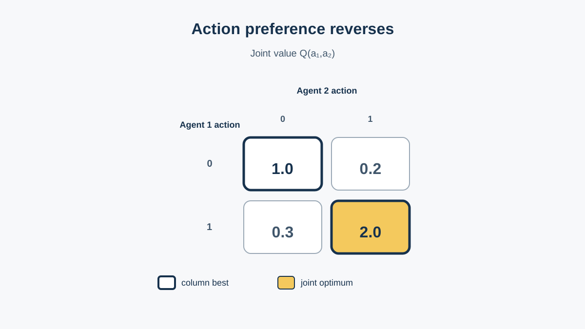
Now the limit. Consider a joint value function where the best joint action requires one agent to take its locally worse action. Concretely: agent 1's utility is higher for action 0 than action 1, but the team's best joint action requires agent 1 to take action 1 because it unlocks a large payoff from agent 2.
In that world, the ordering of agent 1's actions flips depending on what the others do. When agent 2 takes action 0, agent 1 should prefer action 0; when agent 2 takes action 1, agent 1 should prefer action 1. A monotone mixer cannot reproduce that flip. The per-agent ordering is fixed by , and monotonicity preserves it — the mixer can scale the ordering, but it cannot invert it.
Make it concrete with a two-agent, two-action table. Rows are agent 1's action, columns are agent 2's action, and each cell is the true joint value :
| 1.0 | 0.2 | |
| 0.3 | 2.0 |
Read the ordering of agent 1's actions in each column. When agent 2 plays 0, agent 1 prefers 0 (1.0 > 0.3). When agent 2 plays 1, agent 1 prefers 1 (2.0 > 0.2). The preference reverses with the other agent's action. A monotone mixer forces a single ordering of agent 1's actions across both columns, so no choice of and monotone can fit this table. The joint optimum is , but the composed per-agent greedy action under any monotone factorization will land on or — whichever ordering the mixer commits to — never the coordinated cell.
This is a strict limit, and it is worth being precise about where it sits:
- VDN (additive factorization) is a special case of monotone mixing, so monotonicity is strictly more expressive than summation.
- Monotone mixing is still a strict subset of all joint value functions. The table above lives outside it.
There is also a subtler failure mode, the one flagged in the assumptions. If orders an agent's actions incorrectly because cannot see the true state, the mixer cannot repair the ordering. It can only scale a wrong ordering into a wrong joint value. This is a local-observability failure, not a mixing failure, and it is easy to misattribute.
Knowledge check
Check your understanding
Answer this question before you continue.
The Coordination Tradeoff, Stated Plainly
Monotonicity buys a guarantee and cheap maximization. It costs expressiveness on tasks whose optimal coordination is genuinely non-monotonic. That is the trade, and it is not free in either direction.
The practical signal is specific: if your task rewards one agent sacrificing local value for a joint payoff, expect the monotone mixer to underfit and the learned policy to stall at a suboptimal joint action. You will see the team plateau, not diverge — the constraint is stable, just too tight.
You have two responses, and they are not symmetric:
- Keep the constraint and accept the ceiling. You retain IGM by construction and tractable targets. If your task's optimal coordination happens to be monotonic, you lose nothing.
- Relax the constraint and lose the guarantee. Softening monotonicity to a penalty on negative slopes trades the theoretical guarantee for capacity. Decentralized greedy execution is no longer provably optimal — there may exist states where the joint argmax differs from the composed per-agent greedy action.
Common mistake: Treating relaxation as a free upgrade. Relaxing monotonicity does not automatically produce better policies. It trades a guarantee for capacity and adds optimization difficulty. If your task is monotonic, you paid for nothing.
How to Check the Constraint Is Actually Holding
Do not take the guarantee on faith. Measure it.
- Monitor the local partial derivatives. Track during training. Non-negative slopes everywhere means the guarantee is intact.
- Track slope violations if you soften the constraint. Log the frequency and magnitude of negative slopes, and correlate them with episodes where decentralized execution diverges from the joint argmax.
- Run a direct consistency test. On held-out states, compare the composed per-agent greedy action against the joint argmax of . They should match wherever IGM holds.
- Separate consistency from accuracy. A passing consistency check does not mean the factorization is expressive enough. Consistency says the two argmaxes agree; accuracy says the value is right. They are different questions, and a monotone mixer can be perfectly consistent and still wrong.
The Decision Rule
Monotonicity is a guarantee you buy with expressiveness. The right question is not whether the constraint is restrictive — it is restrictive by design — but whether your task's optimal coordination is monotonic. If it is, the constraint is free correctness and free tractability. If it is not, you are paying for a guarantee that does not fit your problem.
The next step is to test that question directly. Take a small cooperative task with a known non-monotonic optimum — one where the best joint action requires an agent to take its locally worse action — and run a monotone mixer against it. Watch where the policy stalls. Then compare against a factorization that targets IGM consistency without the monotone restriction, and measure whether the extra capacity actually buys you the coordination the constraint was forbidding.
Knowledge check
Final check
Finish the article by checking the ideas you just learned.
References
Build a stronger RL mental model
Use structured resources to connect equations, algorithms, and observable agent behavior.


