
Deriving PPO's Clipped Surrogate Objective
You can write PPO's loss in three lines of code and still not know why the min() is there. That gap matters, because the min() is the whole algorithm.

Key topics
You can write PPO's loss in three lines of code and still not know why the min() is there. That gap matters, because the min() is the whole algorithm.
Here is the weak model I want to replace: "clipping keeps the ratio inside [1−ε, 1+ε]." It does not. The ratio can and does sail past the boundary in real training runs. What clipping actually does is remove the incentive to push it further. Once you see that distinction, the objective stops being a ritual and becomes a mechanism you can reason about.
Let's derive it.
What the Ratio Is Actually Measuring
Set the notation once, then leave it alone.
- π_θ(a|s) — the policy you are currently optimizing, with parameters θ.
- π_θold(a|s) — the policy that collected the data sitting in your buffer. Its parameters are frozen.
- r_t(θ) = π_θ(a_t|s_t) / π_θold(a_t|s_t) — the probability ratio.
The ratio is a correction factor. It answers one question: how much more or less likely has this sampled action become under my updated parameters? If r_t > 1, the action got more probable. If r_t < 1, it got less probable. If r_t = 1, nothing has moved yet.
Why do we need a correction factor at all? Because the data came from π_θold, but the expectation we care about is under π_θ. Those are different distributions. Any expectation over π_θ computed from π_θold samples must be reweighted by the ratio. This is importance sampling, and it is not a stylistic choice — it is the price of reusing a batch after the policy has changed.
Where the Ratio Comes From
The reweighting step is short enough to do in full, and doing it removes the main place where readers get stuck.
Suppose you want the expected value of some function f(s, a) under the new policy, but you only have actions sampled from the old policy. For a fixed state s, you can rewrite the expectation by inserting the old policy and cancelling it:
E_{aπ_θ}[f(s, a)] = Σ_a π_θ(a|s) f(s, a) = Σ_a π_θold(a|s) · [π_θ(a|s) / π_θold(a|s)] · f(s, a) = E_{aπ_θold}[ r_t(θ) f(s, a) ]
That is the whole trick. The ratio is the exchange rate between the two distributions. It is valid whenever π_θold assigns nonzero probability to every action you might sample — the support condition. If the old policy never tried an action, you cannot reweight your way to an estimate for it, because you have no samples to reweight.
Now connect f to the policy gradient. The score-function term ∇_θ log π_θ(a_t|s_t) Â_t is exactly the kind of function we want to average under π_θ. Applying the reweighting above gives the likelihood-ratio estimator:
∇_θ J(θ) = E[ r_t(θ) ∇_θ log π_θ(a_t|s_t) Â_t ]
The ratio appears because the score function was reweighted to match the new distribution. Everything below builds on that line.
Note: This reweighting corrects the action distribution at each sampled state. It does not correct the distribution of states themselves. PPO's surrogate keeps states sampled under π_θold and reweights only the actions — a deliberate simplification, not a full trajectory-level correction. Hold that distinction; it explains why the surrogate is a local approximation rather than an exact account of the return.
Knowledge check
Check your understanding
Answer this question before you continue.
From the CPI Objective to the Clipped Surrogate
Drop the gradient and look at the objective it came from. That is the CPI objective (conservative policy iteration):
L_CPI(θ) = E[ r_t(θ) Â_t ]
The expectation here is taken over states sampled by π_θold and actions sampled by π_θold. This is the old-state-distribution surrogate: it holds the state distribution fixed and reweights only the actions. Near r_t ≈ 1, it tracks the true improvement well. Far from it, the approximation degrades — but the objective itself does not know that.
Here is the failure mode. Nothing in L_CPI penalizes a large r_t. If one sampled action carries a big positive advantage, the objective is happy to make that action enormously more likely. One lucky sample, one huge parameter step, one policy that has walked off a cliff. The estimator has no brake.
PPO's fix is to clip the ratio and take the minimum of the clipped and unclipped terms:
L_CLIP(θ) = E[ min( r_t(θ) Â_t, clip(r_t(θ), 1−ε, 1+ε) Â_t ) ]
where ε is a small hyperparameter, commonly around 0.2.
Read the min() as a pessimistic lower bound. For any sample, the objective takes whichever of the two terms is smaller. The unclipped term is the optimistic one — it keeps rewarding the policy for moving further. The clipped term is the cautious one — it stops moving once the ratio leaves the range. Taking the minimum means the objective never pays the policy for going beyond what the clipped term allows.
The subtle part: the min() is not symmetric. Which side of the clip activates depends on the sign of the advantage. That is the next section.
Knowledge check
Check your understanding
Answer this question before you continue.
Reading the Objective by the Sign of the Advantage
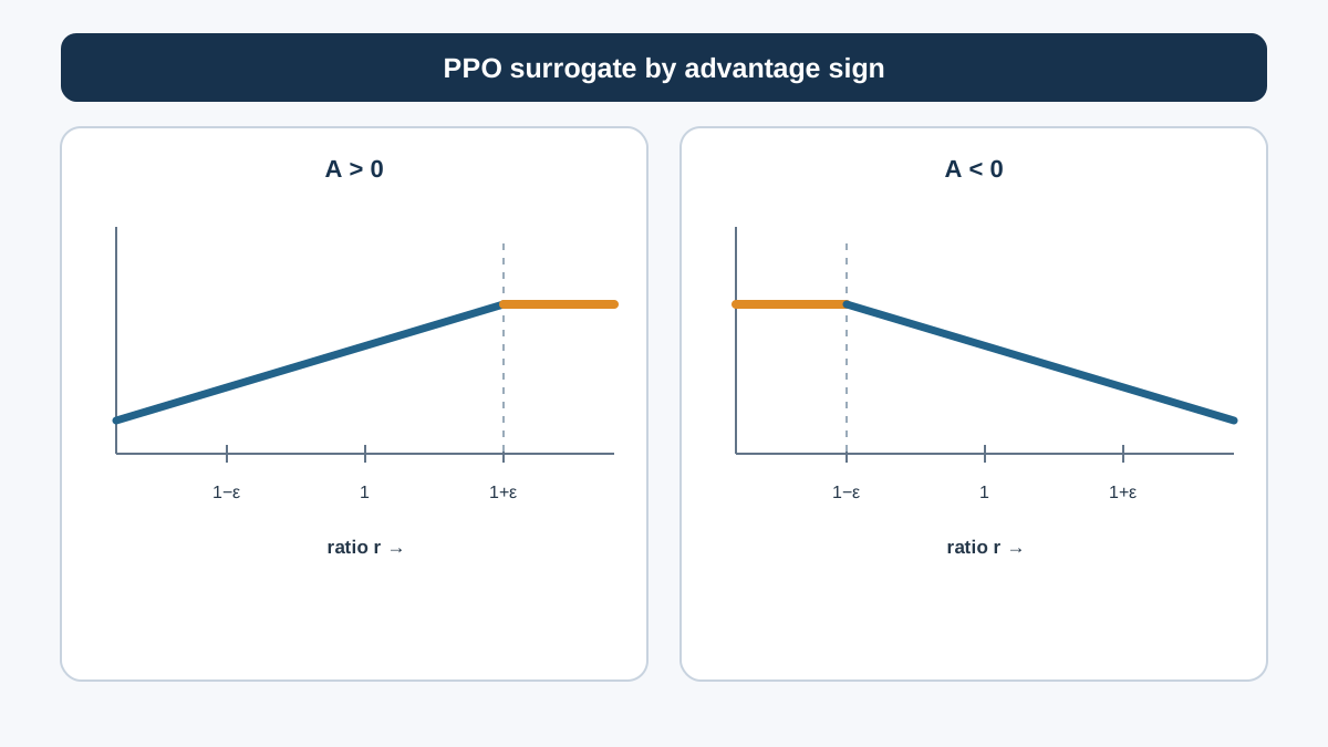
There are four cases, and you can predict all of them from two facts: the sign of Â_t and where r_t sits relative to the clip range.
| Advantage | Ratio position | Active term | Gradient effect |
|---|---|---|---|
| Â_t > 0 | r_t < 1+ε | r_t Â_t | Normal policy gradient — action gets more likely |
| Â_t > 0 | r_t > 1+ε | (1+ε) Â_t | Saturates; gradient contribution goes to zero |
| Â_t < 0 | r_t > 1−ε | r_t Â_t | Action gets less likely, unclipped |
| Â_t < 0 | r_t < 1−ε | (1−ε) Â_t | Saturates; incentive to lower probability disappears |
Walk through the first row. A positive advantage means the action did better than expected, so we want it more likely. As r_t grows, the objective grows with it — ordinary policy gradient. But once r_t crosses 1+ε, the clipped term (1+ε)Â_t is smaller than r_t Â_t, so the min() picks the constant. The objective is now flat in r_t. The gradient from that sample is zero.
The third row is the mirror image. A negative advantage means the action did worse than expected, so we want it less likely. As r_t shrinks, r_t Â_t actually increases (a negative number times a smaller positive number is less negative). The objective rewards lowering the probability — until r_t drops below 1−ε, where the term saturates at (1−ε)Â_t and the incentive vanishes.
Picture two panels of the objective plotted against r_t. For Â_t > 0, the curve rises linearly, then flattens at r_t = 1+ε. For Â_t < 0, it rises as r_t falls, then flattens at r_t = 1−ε. The flat regions are where samples go silent.
Knowledge check
Check your understanding
Answer this question before you continue.
A Worked Example at the Clipping Boundary
Numbers make the flattening visible. Take ε = 0.2, so the clip range is [0.8, 1.2]. Suppose one sample has advantage Â_t = 2.0, and the old policy assigned the action probability 0.5.
Case 1 — ratio inside the range. The new policy assigns probability 0.55, so r_t = 0.55 / 0.5 = 1.1.
- Unclipped term: 1.1 × 2.0 = 2.2
- Clipped term: clip(1.1, 0.8, 1.2) × 2.0 = 1.1 × 2.0 = 2.2
- min(2.2, 2.2) = 2.2
Inside the range, both terms agree. The sample is teaching the policy.
Case 2 — ratio just outside. The new policy assigns probability 0.65, so r_t = 0.65 / 0.5 = 1.3.
- Unclipped term: 1.3 × 2.0 = 2.6
- Clipped term: clip(1.3, 0.8, 1.2) × 2.0 = 1.2 × 2.0 = 2.4
- min(2.6, 2.4) = 2.4
The clipped term wins. The objective is pinned at 2.4.
Case 3 — ratio further outside. The new policy assigns probability 0.75, so r_t = 1.5.
- Unclipped term: 1.5 × 2.0 = 3.0
- Clipped term: 1.2 × 2.0 = 2.4
- min(3.0, 2.4) = 2.4
The objective is still 2.4. The ratio moved from 1.3 to 1.5 — a real change in the policy — but the objective did not budge. That sample now contributes zero gradient in the direction that would push the ratio higher.
Common mistake: Reading this as "the ratio is capped at 1.2." It is not. The ratio in case 3 is 1.5, and nothing in the objective prevents it from reaching 2.0 or 10.0. What the objective removes is the reward for going there. The policy can still drift; it just stops being paid for it.
Knowledge check
Check your understanding
Answer this question before you continue.
What the Objective Assumes and What It Does Not Guarantee
The clipped surrogate is a local approximation, and its guarantees are narrower than they look.
It is informative near r_t ≈ 1. The CPI objective approximates the true improvement well when the new policy is close to the data-collecting policy. As the ratio drifts, the approximation degrades, and the clipped objective inherits that degradation. Clipping slows the drift; it does not repair the approximation.
Clipping bounds the incentive, not the KL divergence. These are related but not equivalent. A policy can accumulate a large KL divergence from θold while every individual sample sits comfortably inside the clip range. The clip range constrains per-sample movement, not the aggregate distance between distributions.
Advantage quality is an input assumption. The objective is only as good as Â_t. A noisy or biased advantage estimate makes the clipped objective confidently wrong — it will stabilize the policy around a bad signal. Garbage in, stable garbage out.
Multiple epochs push the ratio outward. PPO typically optimizes the same batch for several epochs. Each epoch moves θ further from θold, so ratios drift toward and past the boundary. This is why implementations add early stopping on measured KL divergence: when the mean KL between new and old policies exceeds a threshold, stop taking gradient steps on that batch.
It is a heuristic, not a proof. TRPO came with a monotonic-improvement argument under specific conditions. PPO's clipped objective has strong empirical support and a clean intuition, but it does not carry the same theoretical guarantee. Treat it as a well-tested stabilization device.
When This Objective Is the Right Tool
The clipped surrogate fits when three conditions hold: the data is on-policy (collected by π_θold and used soon after), the policy is stochastic, and you want a simple first-order update that tolerates some drift.
It fits poorly when you want heavy off-policy reuse. The ratio correction becomes unreliable when the data-collecting policy is far from the current one, and the clip range stops meaning anything useful.
Two quick comparisons:
- Against a hard trust-region constraint (TRPO): TRPO enforces a KL constraint with a second-order method. PPO replaces that with a first-order penalty you can run with plain SGD. You trade a formal guarantee for implementation simplicity.
- Against unclipped policy gradient: You remove the brake entirely. Updates are faster when they are right and catastrophic when they are wrong.
The tuning reality: ε trades update aggressiveness against stability, and the useful range is narrow — commonly cited values sit between 0.1 and 0.3. Set it too high and you are back to unclipped behavior; too low and the policy barely moves.
Every knob here is a direct consequence of a term in the objective. That is the payoff of the derivation.
Where to Go Next
When you read a PPO loss, check two things first: the sign of the advantage and the position of the ratio. Those two facts tell you whether a sample is still teaching the policy or has gone silent.
Then instrument it. Log the clip fraction — the share of samples whose ratio falls outside [1−ε, 1+ε] — and the mean KL divergence between the new and old policies during a short training run. Watch the clip fraction rise across epochs on the same batch. Watch the KL cross your early-stopping threshold. The boundary stops being algebra and becomes a number on a chart, moving in real time.
Knowledge check
Final check
Finish the article by checking the ideas you just learned.
References
Build a stronger RL mental model
Use structured resources to connect equations, algorithms, and observable agent behavior.


