Implement a Small PPO Learner in Python

You can read PPO's clipped objective ten times and still not know whether your implementation works. The curve tells you. So does the clip fraction. So does the moment your advantage estimates quietly go to zero.

This is a build article. We will write a single-file PPO learner on CartPole-v1, run it, and read the diagnostics that separate "the script ran" from "the agent learned." Then we will change exactly one thing and watch what happens.

What You Are Building and What It Must Prove

The learner has four moving parts: an MLP actor-critic, a rollout collector, a GAE-style advantage estimator, and a clipped surrogate update that runs several epochs over one frozen batch. That is the whole algorithm. Everything else is plumbing.

Dependencies are minimal: Python, PyTorch, and Gymnasium. CartPole-v1 is the benchmark because episodes are short, returns are integers you can eyeball, and a correct learner usually solves it in a few hundred updates.

Success means three things at once:

• Episode return trends upward. Noisy, but upward.
• Policy loss and value loss stay finite. No NaN, no explosion.
• Approximate KL and clip fraction stay in a sane band — small but nonzero.

Explicit non-goals: no vectorized environments, no distributed training, no hyperparameter search. Those are later concerns. If you add them now, you will not know which change broke the run.

The Loop Skeleton: Collect, Estimate, Update

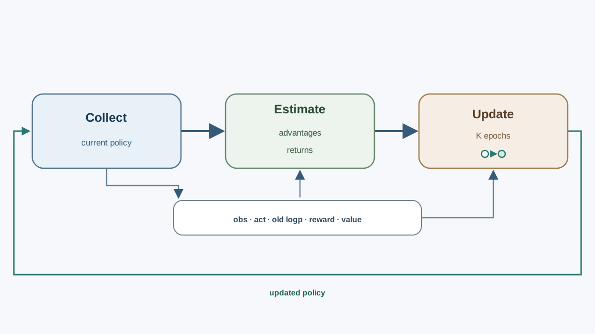
Every PPO iteration has three phases, in this order:

1. Collect. Roll out the current policy for N steps. Store states, actions, log-probabilities, rewards, episode boundaries, and value estimates.
2. Estimate. Compute discounted returns and advantages from that batch.
3. Update. Run K epochs of minibatch gradient steps on the same frozen batch.

That third point is the one beginners skip past. PPO's ratio compares the new policy against the behavior policy that produced the data. If you keep collecting during the update, the denominator drifts and the ratio stops meaning what the math says it means. Freeze the batch. Then learn from it.

The actor and critic share a trunk — a couple of linear layers — and split into two heads: one producing action logits, one producing a scalar value. Shared features, separate targets.

Step 1: Environment and Rollout Collection

Gymnasium's API returns five values from step: observation, reward, terminated, truncated, info. The terminated vs truncated distinction matters. A truncated episode hit a time limit; the state is not terminal, so you should bootstrap from it. A terminated episode is genuinely over.

The subtle part is that both cases reset the environment, but only one of them should stop the advantage trace. Store them as two separate flags so the estimator can tell them apart.

import torch
import torch.nn as nn
import gymnasium as gym

class ActorCritic(nn.Module):
    def __init__(self, obs_dim, act_dim, hidden=64):
        super().__init__()
        self.trunk = nn.Sequential(
            nn.Linear(obs_dim, hidden), nn.Tanh(),
            nn.Linear(hidden, hidden), nn.Tanh(),
        )
        self.actor = nn.Linear(hidden, act_dim)
        self.critic = nn.Linear(hidden, 1)

    def forward(self, x):
        h = self.trunk(x)
        return self.actor(h), self.critic(h).squeeze(-1)

The rollout function stores log_prob at action time. This is the behavior-policy record the ratio later divides by. Recomputing it later is a bug, not an optimization.

def collect_rollout(env, model, steps=2048):
    obs, _ = env.reset()
    data = {k: [] for k in
            ["obs", "act", "logp", "rew", "term", "trunc", "val"]}
    ep_returns, ep_ret = [], 0.0
    for _ in range(steps):
        obs_t = torch.as_tensor(obs, dtype=torch.float32)
        with torch.no_grad():
            logits, value = model(obs_t)
            dist = torch.distributions.Categorical(logits=logits)
            action = dist.sample()
            logp = dist.log_prob(action)
        next_obs, reward, term, trunc, _ = env.step(action.item())
        data["obs"].append(obs_t)
        data["act"].append(action)
        data["logp"].append(logp)
        data["rew"].append(reward)
        data["term"].append(term)
        data["trunc"].append(trunc)
        data["val"].append(value)
        ep_ret += reward
        obs = next_obs
        if term or trunc:
            ep_returns.append(ep_ret)
            ep_ret = 0.0
            obs, _ = env.reset()
    return data, ep_returns, obs

Print the batch shape and the raw episode returns before you train anything. If the untrained policy scores around 20 on CartPole, your environment wiring is correct.

Step 2: Advantages and Returns Without the Confusion

This is where most implementations break. Three quantities, three different jobs:

• Reward is what the environment handed you at one step.
• Return is the discounted sum of future rewards from that step.
• Advantage is the return minus the value estimate — how much better the outcome was than the critic expected.

The advantage trace must stop at a true termination, but it must not stop at a truncation. At a truncation, the episode ended because of a time limit, not because the state is dead. So the trace continues, bootstrapping from the value of the final observation — not the value of the reset observation.

def compute_gae(data, last_obs, model, gamma=0.99, lam=0.95):
    with torch.no_grad():
        _, last_val = model(torch.as_tensor(last_obs, dtype=torch.float32))
    rewards = data["rew"]
    values = data["val"] + [last_val]
    terms = data["term"] + [False]
    truncs = data["trunc"] + [False]
    adv, gae = [], 0.0
    for t in reversed(range(len(rewards))):
        # A true termination kills the trace. A truncation does not.
        alive = 0.0 if terms[t] else 1.0
        # Bootstrap from the next value only if the next step is real.
        next_val = values[t + 1] if not (terms[t] or truncs[t]) else 0.0
        delta = rewards[t] + gamma * next_val - values[t]
        gae = delta + gamma * lam * alive * gae
        adv.insert(0, gae)
    adv = torch.stack(adv)
    returns = adv + torch.stack(data["val"])
    adv = (adv - adv.mean()) / (adv.std() + 1e-8)
    return adv, returns

The critic regresses on returns. The actor is weighted by advantages. Two different targets, one shared trunk.

Common mistake: If your advantages are all near zero or wildly large, you have a boundary bug or a normalization bug — not a bad learning rate. Check the term and trunc masks first. The most common version of this bug is treating truncation as termination, which throws away the bootstrap value at every time-limit boundary and biases the critic toward pessimism.

Step 3: The Clipped Update in Code

The ratio is the exponentiated difference between new and old log-probabilities. The clipped surrogate takes the minimum of the unclipped and clipped terms. The update also computes the two diagnostics you will read later: approximate KL and clip fraction.

def update(model, opt, data, adv, returns, epochs=10, clip=0.2):
    obs = torch.stack(data["obs"])
    act = torch.stack(data["act"])
    old_logp = torch.stack(data["logp"]).detach()
    n = len(obs)
    kl_sum, clip_sum, batches = 0.0, 0.0, 0
    for _ in range(epochs):
        idx = torch.randperm(n)
        for start in range(0, n, 256):
            mb = idx[start:start+256]
            logits, value = model(obs[mb])
            dist = torch.distributions.Categorical(logits=logits)
            logp = dist.log_prob(act[mb])
            ratio = torch.exp(logp - old_logp[mb])
            surr1 = ratio * adv[mb]
            surr2 = torch.clamp(ratio, 1-clip, 1+clip) * adv[mb]
            policy_loss = -torch.min(surr1, surr2).mean()
            value_loss = ((value - returns[mb]) ** 2).mean()
            entropy = dist.entropy().mean()
            loss = policy_loss + 0.5 * value_loss - 0.01 * entropy
            opt.zero_grad()
            loss.backward()
            opt.step()
            with torch.no_grad():
                kl_sum += (old_logp[mb] - logp).mean().item()
                clip_sum += ((ratio - 1.0).abs() > clip).float().mean().item()
                batches += 1
    return kl_sum / batches, clip_sum / batches

Three terms, three jobs. Policy loss pushes probability toward actions with positive advantage. Value loss trains the critic. Entropy keeps the policy from collapsing to one action too early. The coefficients trade off: raise the value coefficient and the critic learns faster but the actor moves slower.

Print the mean ratio on the first epoch. It should be near 1.0 — the policy has not changed yet. By the last epoch it should have drifted, but not far. If it hits 3.0, your update is too aggressive.

Step 4: The Training Loop That Actually Runs

Now assemble the pieces. The loop collects a batch, computes advantages, runs the update, and prints the diagnostics you will read.

def train(total_updates=300, rollout_steps=2048):
    env = gym.make("CartPole-v1")
    obs_dim = env.observation_space.shape[0]
    act_dim = env.action_space.n
    model = ActorCritic(obs_dim, act_dim)
    opt = torch.optim.Adam(model.parameters(), lr=3e-4)
    recent_returns = []
    for it in range(total_updates):
        data, ep_returns, last_obs = collect_rollout(env, model, rollout_steps)
        adv, returns = compute_gae(data, last_obs, model)
        kl, clip_frac = update(model, opt, data, adv, returns)
        recent_returns.extend(ep_returns)
        recent_returns = recent_returns[-100:]
        mean_ret = sum(recent_returns) / max(len(recent_returns), 1)
        print(f"update {it:3d} | return {mean_ret:6.1f} | "
              f"kl {kl:.4f} | clip {clip_frac:.3f} | "
              f"eps {len(ep_returns)}")
    env.close()

if __name__ == "__main__":
    train()

Run it:

pip install torch gymnasium
python ppo_cartpole.py

What you should see: the return column climbs from around 20 toward 200 over a few hundred updates, with visible noise. The KL column stays small — roughly 0.005 to 0.02. The clip fraction stays in the 0.05 to 0.2 band. If any of those three numbers leaves its band, you have a specific bug to chase, not a vague "it's not learning."

Reading the Diagnostics: Is It Actually Learning?

A script that runs without crashing has proven nothing. Read these four numbers:

Diagnostic	Healthy	Too aggressive	Too timid
Episode return	Noisy rise	Spikes then collapses	Flat
Approximate KL	0.005–0.02	> 0.05	~ 0
Clip fraction	0.05–0.2	> 0.4	~ 0
Value loss	Decreasing	Diverging	Stuck high

Expect a noisy rise, not a smooth line. CartPole returns bounce between 9 and 200 even after the agent has essentially solved the task. Judge over 50–100 episodes, not 5.

Warning: Do not tune on a single lucky run. Run three seeds with the same hyperparameters. If the variance between seeds is larger than the effect you are chasing, you are reading noise.

Common Failure Modes and How to Debug Them

Flat return curve, near-zero clip fraction. The policy is not moving. Either the learning rate is too low, the advantages are miscomputed, or the policy has collapsed to a single action (check entropy — if it is near zero, the entropy bonus is too small).

Return collapses after an early rise. The update is too large. Cut the number of epochs per batch, lower the learning rate, or verify advantage normalization is actually running.

Value loss diverges while policy loss looks fine. The critic is chasing targets that scale badly. Check that returns are not exploding, and consider a separate, smaller learning rate for the value head.

Silent bug worth naming. If you forget to .detach() the old log-probs and values, the ratio's denominator carries gradient. The loss still decreases. The policy still changes. But the ratio is now measuring something else, and the clipping guarantee is gone. Detach the behavior-policy record.

Truncation treated as termination. If you collapse term and trunc into a single done flag, the advantage trace stops at every time-limit boundary. The critic learns to expect the episode to end, and the policy becomes pessimistic about long-horizon returns. This is the bug the two-flag representation in Step 1 exists to prevent.

One Bounded Modification: Change the Entropy Coefficient

Now the experiment. Change exactly one number: the entropy coefficient, currently 0.01.

• Raise it to 0.05 to encourage exploration.
• Lower it to 0.001 to let the policy sharpen.

State the prediction before you run. Higher entropy should slow early return growth — the policy spends probability on actions it does not yet trust — but it should also reduce the chance of collapsing to a single action. Lower entropy should sharpen faster but risk premature commitment.

Keep everything else fixed. Compare the same diagnostic panel across runs.

What the result teaches: entropy is an exploration dial, not a performance dial. Its right value depends on how much the task rewards commitment. CartPole rewards a decisive push in one direction; a task with sparse rewards and many dead ends rewards lingering exploration. The coefficient is a statement about the task, not a knob to maximize.

Where This Goes Next

The learner you built is not a finished algorithm. It is a diagnostic harness. The same collect-estimate-update skeleton, the same four-number panel, and the same one-change-at-a-time discipline scale to harder problems.

The natural next step: swap CartPole for a continuous-control task like Pendulum-v1. The action space changes from discrete to Gaussian, the actor head outputs a mean and log-standard-deviation, and the log-probability computation changes shape. Watch which diagnostic breaks first — usually the value loss, because continuous returns have a wider range.

Here is the decision rule I would keep: when a run fails, read the diagnostics before touching the hyperparameters. The numbers tell you which part of the loop is lying to you. The hyperparameters only tell you how loudly.