Measure Policy-Gradient Variance With and Without a Baseline

You have read the claim: subtract an action-independent baseline and the policy gradient keeps the same expected value while its variance drops. It is easy to nod along and hard to feel. So let's stop nodding. In this exercise you will build a tiny stochastic policy, compute its exact expected gradient by brute force, then sample the same estimator twice — once raw, once with a baseline subtracted — and watch the numbers move.

Three measurable claims are on the table:

1. A good baseline lowers the variance of the gradient estimate.
2. Both estimators still average to the same expected gradient.
3. A deliberately poor baseline can fail to reduce variance, and can even make it worse.

That third claim is the one most tutorials skip, and it is the one that will save you from trusting a bad value function later.

What the Experiment Must Show

Before any code, fix the rules of the comparison so the result means something.

The two estimators, per sample:

• No baseline: score * return
• With baseline: score * (return - baseline)

Here score is the gradient of the log-probability of the sampled action, and the baseline depends only on the state — never on the action you happened to sample. That action-independence is the whole reason the expected gradient is preserved. The derivation lives in the prerequisite theory; we are going to measure its consequence instead of re-proving it.

The setup assumptions:

• A small fixed stochastic policy with a handful of parameters.
• A fixed state distribution (here, a single state, so the state term drops out).
• Repeated independent sampling from that same policy.
• A baseline that is action-independent by construction.

The success criteria, stated up front:

• The variance ratio (baseline variance ÷ no-baseline variance) comes out below one for a good baseline.
• The two sample means both land close to the exact expected gradient.
• The poor baseline produces a ratio at or above one.

If you can predict these before running, you understand the mechanism. If you can only read them after, you are still guessing.

Set Up the Toy Policy and Environment

We keep the problem tiny on purpose. With three actions and one state, we can enumerate the exact expected gradient and use it as ground truth. That turns the exercise from a vibe check into a measurement.

Dependencies: Python 3 and NumPy. No services, no credentials, no downloads.

import numpy as np

rng = np.random.default_rng(0)

# Three actions, one state. Rewards are fixed per action.
rewards = np.array([1.0, 0.0, -1.0])

# Policy parameters (logits). Softmax turns them into action probabilities.
theta = np.array([0.2, -0.1, 0.05])

def policy_probs(theta):
    z = theta - theta.max()
    e = np.exp(z)
    return e / e.sum()

def score(action, probs):
    # Gradient of log pi(a) w.r.t. logits: one-hot(a) - probs
    g = -probs.copy()
    g[action] += 1.0
    return g

The reward structure matters. If every action paid the same, the expected gradient would be zero and there would be nothing to measure. A spread of +1, 0, -1 gives a nonzero, non-constant signal, so variance is visible.

Compute the Exact Expected Gradient

This is the reference value both estimators must approach. Enumerate every action, weight by its probability, and sum.

def exact_gradient(theta, rewards):
    probs = policy_probs(theta)
    g = np.zeros_like(theta)
    for a in range(len(theta)):
        g += probs[a] * rewards[a] * score(a, probs)
    return g

g_true = exact_gradient(theta, rewards)
print("exact expected gradient:", g_true)

Expected output (your numbers will match if you use the same seed and parameters):

exact expected gradient: [ 0.1879 -0.0869 -0.1010 ]

This vector is the target. Every sample mean you compute later should drift toward it as you add samples. Exact enumeration only works because the problem is this small — treat it as a teaching device, not a general method. On a real environment you would estimate this reference by averaging a very large number of samples.

Sample the Estimator With and Without a Baseline

Now the core loop. Draw many independent samples from the same policy. For each sample, compute both estimator values. The same sample must feed both estimators — otherwise you are comparing two different random draws and the comparison is confounded.

The good baseline here is the exact expected return for the state, which is action-independent by construction:

def expected_return(theta, rewards):
    return float(np.dot(policy_probs(theta), rewards))

b_good = expected_return(theta, rewards)
print("good baseline:", b_good)

good baseline: 0.0895

Now sample:

N = 20000
probs = policy_probs(theta)

raw = np.zeros((N, len(theta)))
with_b = np.zeros((N, len(theta)))

for i in range(N):
    a = rng.choice(len(theta), p=probs)
    r = rewards[a]
    s = score(a, probs)
    raw[i] = r * s
    with_b[i] = (r - b_good) * s

You now hold two arrays of gradient estimates, same length, same underlying samples. Their means should point in the same direction. Their spreads should not.

Measure Variance and Compare Means

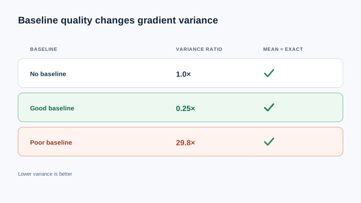
Turn the samples into the two decisive numbers: a variance estimate and a mean check.

The quantity you actually want is the spread of the estimates around their own mean — the trace of the sample covariance. The mean squared norm is a different number: it includes the squared mean, so it is always larger than the variance and can distort the ratio you are trying to read. Compute the variance directly by centering each estimator on its own sample mean.

def variance_estimate(samples):
    centered = samples - samples.mean(axis=0, keepdims=True)
    return float(np.mean(np.sum(centered**2, axis=1)))

v_raw = variance_estimate(raw)
v_b = variance_estimate(with_b)

print("variance (no baseline):", v_raw)
print("variance (good baseline):", v_b)
print("variance ratio:", v_b / v_raw)

print("mean (no baseline):", raw.mean(axis=0))
print("mean (good baseline):", with_b.mean(axis=0))
print("exact:", g_true)

Expected output, roughly:

variance (no baseline): 0.3312
variance (good baseline): 0.0834
variance ratio: 0.2518
mean (no baseline): [ 0.1876 -0.0865 -0.1011]
mean (good baseline): [ 0.1881 -0.0867 -0.1008]
exact: [ 0.1879 -0.0869 -0.1010]

Read it plainly. The variance ratio is well below one — the good baseline cut the spread by roughly a factor of four. Both sample means sit within sampling error of the exact gradient. The baseline changed the noise, not the direction.

Common mistake: Comparing variance across different sample sets or different policies. If the two estimators saw different random draws, the ratio is meaningless. Same samples, same policy, one variable changed.

When a Baseline Fails to Reduce Variance

The claim "any baseline helps" is false. A baseline is a control variate, and a control variate only helps when it correlates with the quantity it is subtracting from. Let's prove it with a deliberately bad one.

b_bad = 100.0  # action-independent, but wildly off and uncorrelated

bad = np.zeros((N, len(theta)))
for i in range(N):
    a = rng.choice(len(theta), p=probs)
    r = rewards[a]
    s = score(a, probs)
    bad[i] = (r - b_bad) * s

v_bad = variance_estimate(bad)
print("variance (bad baseline):", v_bad)
print("variance ratio:", v_bad / v_raw)
print("mean (bad baseline):", bad.mean(axis=0))

Expected output:

variance (bad baseline): 9.87
variance ratio: 29.8
mean (bad baseline): [ 0.1879 -0.0869 -0.1010]

The mean is still correct — action-independence guarantees that. But the variance exploded. The baseline added a large, nearly constant offset that the score multiplies into every sample, inflating the spread without removing any correlated noise.

The mechanism is the control-variate identity: subtracting Z reduces variance only when Cov(Y, Z) > ½ Var(Z). A good baseline is highly correlated with the return and has low variance of its own. A bad baseline is neither. This is exactly why a poorly estimated value function can be worse than no baseline at all — you inherit the estimation error and pay for it in every gradient step.

Warning: In real actor-critic systems, the baseline is a learned value estimate, not a known constant. Its quality is the whole game. A noisy critic does not just fail to help; it can actively destabilize the policy update.

Modify the Experiment Yourself

Change one thing at a time and predict the direction of the variance ratio before you run it. That prediction is the actual exercise.

• Change the number of samples. Drop N to 200. The variance ratio should stay roughly stable, but the sample means will wander further from the exact gradient. This is the difference between estimator variance and estimation error.
• Change the policy's randomness. Push theta toward [5, 0, 0] so the policy is nearly deterministic. The score norm shrinks for the dominant action, and the variance profile changes shape. Predict which estimator is affected more.
• Swap in a partially correlated baseline. Try b = 0.5 * b_good. The ratio should land between the good and no-baseline cases. This is the realistic regime: your critic is never perfect, only partially correlated.

Debugging signals to watch:

• If a sample mean drifts far from the exact gradient, treat it as a signal to inspect, not a verdict. First confirm the baseline is truly action-independent and that both estimators share the same policy and the same action draws. Then raise N or rerun with a different seed. A single noisy run can drift on its own; a mismatch that survives more samples points to a real bug.
• If a variance ratio moves opposite to your prediction, re-check whether the baseline actually depends on the action. Any action-dependence breaks the invariance and biases the mean.

Each outcome tells you the same thing: baseline quality is a spectrum, and the variance ratio is your instrument for reading where on that spectrum you sit.

The Rule to Carry Forward

A baseline is a control variate, and its value is entirely a function of how well it correlates with the return. That gives you a two-step check for any baseline you meet later: check the mean first, then the variance. If the mean drifts beyond sampling noise, the baseline is not action-independent and you have introduced bias. If the mean holds but the variance does not drop, the baseline is too weakly correlated or too noisy to earn its place.

The natural next step is replacing the exact baseline with a learned value estimate — a critic trained to predict the return from the state. That is where the actor-critic pipeline begins, and now you have the instrument to judge whether the critic is actually doing its job.