Run a Policy-Gradient Experiment in CartPole With PyTorch

Your loss goes down. Your code runs clean. The pole still falls.

That gap between a falling loss and a falling pole is the first thing to fix, because it tells you which number you are actually watching. In a policy-gradient run, the loss is not a score. It is a weighted sum of log-probabilities, and it can drift in either direction while the policy gets better. The scoreboard is the episode return curve, read across more than one seed.

This tutorial builds the smallest honest REINFORCE learner for CartPole, runs it end to end, and reads the output like an experiment. If you have not yet worked through the derivation of the likelihood-ratio estimator, the short version is enough to proceed: sample an action, record its log-probability, weight that log-probability by the return that followed, and push the parameters in the direction that makes good outcomes more likely. Here we turn that estimator into a training loop that actually produces numbers.

What You Are Actually Building

The agent is a small multilayer perceptron that maps CartPole's four observations — cart position, cart velocity, pole angle, pole angular velocity — to a probability over two actions: push left or push right. The policy is stochastic by design. It samples actions rather than taking the argmax, because the sampling is what generates the exploration the estimator needs.

Before writing a line, state your success criteria:

• Mean episode return climbs well above the random baseline (roughly 20 steps) and keeps climbing.
• Evaluation episodes are consistent across seeds, not a single lucky run.
• The learning curve is readable: flat, then climbing, with visible variance.

And state the non-goals. This is not PPO, not actor-critic, not a benchmark comparison. It is the smallest loop that demonstrates credit assignment through sampled returns. Everything else is a later article.

Environment and Dependencies

Pin the stack in one virtual environment so the RL library and the tensor library share an interpreter:

python -m venv .venv
source .venv/bin/activate      # Windows: .venv\Scripts\activate
pip install "gymnasium[classic-control]" numpy torch

Python 3.10 or newer is a reasonable floor. Keep rendering off during training — it slows runs and adds nothing to the numbers.

The Gymnasium API shape matters here, and it is a silent bug source if you carry over habits from the older Gym API. reset() returns a tuple of (observation, info). step() returns a five-tuple: observation, reward, terminated, truncated, info. The split between terminated and truncated is not cosmetic — one means the episode ended naturally, the other means a time limit cut it off. Treating them as one flag is a common way to corrupt your returns.

Run a random-action rollout before any learning code exists. This is the baseline every later number is compared against:

import gymnasium as gym

env = gym.make("CartPole-v1")
obs, info = env.reset(seed=0)
episode_length = 0

while True:
    action = env.action_space.sample()
    obs, reward, terminated, truncated, info = env.step(action)
    episode_length += 1
    if terminated or truncated:
        break

print("random episode length:", episode_length)

Expect roughly 10 to 25 steps. If you see that, the environment works and your baseline is real.

The Policy Network and Action Sampling

The network ends in raw logits. Do not apply softmax yourself and then feed probabilities into a distribution — that applies the transform twice and quietly distorts the gradient.

import torch
import torch.nn as nn
from torch.distributions import Categorical

class Policy(nn.Module):
    def __init__(self, obs_dim=4, n_actions=2, hidden=64):
        super().__init__()
        self.net = nn.Sequential(
            nn.Linear(obs_dim, hidden),
            nn.ReLU(),
            nn.Linear(hidden, n_actions),
        )

    def forward(self, obs):
        return self.net(obs)

    def act(self, obs):
        logits = self.forward(obs)
        dist = Categorical(logits=logits)
        action = dist.sample()
        return action, dist.log_prob(action)

Categorical(logits=...) handles the softmax internally. The call to dist.log_prob(action) is the likelihood-ratio term from the derivation made concrete: it is the log of the probability your policy assigned to the action it actually took.

The critical detail is what you store. Keep the live log-probability tensor — the one still attached to the graph. If you call .detach(), or rebuild the tensor from a stored integer action, you sever the gradient path and the agent will not learn no matter how long you train. This is the single most common silent failure in a from-scratch implementation.

Print one distribution to confirm the policy starts near-uniform:

policy = Policy()
obs_t = torch.tensor(obs, dtype=torch.float32)
print(torch.softmax(policy(obs_t), dim=-1))

You should see something close to [0.5, 0.5]. That is the correct starting point — an untrained policy should not prefer either action.

Collecting an Episode and Computing Returns

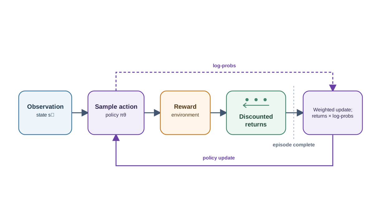
Roll out one full episode, storing log-probabilities and rewards per step. Then compute discounted returns by walking the reward list backward — the linear-time trick:

def run_episode(env, policy, gamma=0.99):
    obs, _ = env.reset()
    log_probs, rewards = [], []

    while True:
        obs_t = torch.tensor(obs, dtype=torch.float32)
        action, log_prob = policy.act(obs_t)
        obs, reward, terminated, truncated, _ = env.step(action.item())

        log_probs.append(log_prob)
        rewards.append(reward)

        if terminated or truncated:
            break

    returns = []
    running = 0.0
    for r in reversed(rewards):
        running = r + gamma * running
        returns.append(running)
    returns.reverse()

    return log_probs, returns

Why backward? Because the return at step t depends on every reward after it. Walking forward would force you to recompute the tail at each step; walking backward carries one running sum and finishes in a single pass.

REINFORCE is Monte Carlo: the update waits for the whole episode. That is why credit assignment is delayed and noisy — a good action early in a long episode gets credited partly for luck that arrived later.

The Update: Why the Loss Number Lies

The objective is the negative sum of log-probabilities weighted by returns. Normalize the returns first — subtract the mean and divide by the standard deviation:

import numpy as np

def update(policy, optimizer, log_probs, returns, gamma=0.99):
    returns_t = torch.tensor(returns, dtype=torch.float32)
    returns_t = (returns_t - returns_t.mean()) / (returns_t.std() + 1e-8)

    loss = 0.0
    for log_prob, ret in zip(log_probs, returns_t):
        loss += -log_prob * ret

    optimizer.zero_grad()
    loss.backward()
    optimizer.step()
    return loss.item()

The sign flip turns gradient ascent on expected return into a minimization call. That is the only reason the word "loss" appears.

Normalization is a variance-reduction step, not a learned critic. It rescales the learning signal so that a single episode's raw return magnitude does not dominate the gradient. Keep the distinction clear: a baseline is a fixed or running statistic; a critic is a learned function. We are doing the former.

Here is the part that trips people up. The reported loss is not a quality metric. It is a weighted sum of log-probabilities, and it can move in either direction while the policy improves. If you watch it like a supervised training loss, you will draw the wrong conclusion at the wrong time.

Scale matters too. Raw returns of 10 to 500 multiply the log-probability gradient, so learning rate and return normalization interact. Normalize the returns and a moderate learning rate behaves predictably; skip normalization and you may need a much smaller rate to avoid blowing up the policy.

Assembling the Full Training Run

Now wire the pieces together. This driver trains for a fixed number of episodes, records each episode's return, and prints a moving average so you can watch the curve take shape:

def train(seed, episodes=500, gamma=0.99, lr=1e-2, window=20):
    torch.manual_seed(seed)
    env = gym.make("CartPole-v1")
    env.reset(seed=seed)

    policy = Policy()
    optimizer = torch.optim.Adam(policy.parameters(), lr=lr)
    history = []

    for ep in range(episodes):
        log_probs, returns = run_episode(env, policy, gamma)
        update(policy, optimizer, log_probs, returns, gamma)
        history.append(sum(returns))

        if (ep + 1) % 50 == 0:
            recent = np.mean(history[-window:])
            print(f"seed {seed} | episode {ep + 1} | mean return {recent:.1f}")

    env.close()
    return history

Run it for three seeds and keep the histories:

histories = {seed: train(seed) for seed in (0, 1, 2)}

A healthy run prints a mean return that starts near the random baseline and climbs into the hundreds. If all three seeds stay near 20, do not train longer — debug. The next section tells you where to look.

Reading the Return Curve

Plot or print the mean episode return over a moving window. Single-episode returns are too noisy to read — a lucky episode can look like progress and a bad one can look like collapse.

Run at least three seeds and overlay them. REINFORCE on CartPole is high variance, and one lucky run proves nothing. If seed 0 solves the task and seeds 1 and 2 stay flat, you have a variance problem, not a solution.

Separate training returns from evaluation returns. During evaluation, run the policy greedily with no learning, so you see the actual policy rather than the exploration noise:

def evaluate(policy, env, episodes=20):
    total = 0
    for _ in range(episodes):
        obs, _ = env.reset()
        while True:
            obs_t = torch.tensor(obs, dtype=torch.float32)
            with torch.no_grad():
                action = policy(obs_t).argmax().item()
            obs, reward, terminated, truncated, _ = env.step(action)
            total += reward
            if terminated or truncated:
                break
    return total / episodes

Expect a flat-then-climb shape. A curve that never leaves the random baseline is a signal to debug, not to train longer.

Diagnosing a Stalled Run

The most common failure is an agent that stays at random performance. Work through these checks in order.

Check the gradient path first. Confirm your log-probabilities carry grad_fn and that the loss is not built from detached tensors. If you converted actions to a tensor and re-encoded them, the gradient is gone.

Check the API. Verify terminated and truncated are both handled, and that the episode actually resets. A loop that never resets will produce nonsense returns.

Check scale. A learning rate that is too high collapses the policy to one action within a few episodes. One that is too low looks like no learning at all.

Watch the action distribution. This is the diagnostic the training loop above does not yet print, so add it. Every fifty episodes, log the mean softmax probability the policy assigns to each action across a batch of observations:

def action_probs(policy, env, samples=200):
    obs_batch = []
    obs, _ = env.reset()
    for _ in range(samples):
        obs_batch.append(obs)
        action = env.action_space.sample()
        obs, _, terminated, truncated, _ = env.step(action)
        if terminated or truncated:
            obs, _ = env.reset()
    obs_t = torch.tensor(np.array(obs_batch), dtype=torch.float32)
    with torch.no_grad():
        probs = torch.softmax(policy(obs_t), dim=-1).mean(dim=0)
    return probs

Call it inside the training loop and print the result. A policy that has collapsed to [1.0, 0.0] has stopped exploring, and plain REINFORCE will not recover from that on its own — the samples it needs to correct the mistake are the samples it no longer takes. A healthy policy keeps both actions in play while it learns.

If the run is still flat after these checks, the fix is usually variance reduction — a baseline or an actor-critic — not more episodes. More episodes of the same noisy estimator just gives you more of the same noise.

One Experiment to Run Next

Add a constant or running-mean baseline subtracted from the returns, and compare the return curves across the same seeds.

Predict the outcome before you run it: the expected update direction is unchanged, but the variance is lower, so the climb should be faster and steadier. If your prediction is wrong, that is evidence about the mechanism, not a personal failure.

Keep the comparison honest — same seeds, same episode budget, same evaluation procedure. Then note what you have actually built: that baseline is the seed of the critic in actor-critic methods. The next conceptual step is not a new topic. It is the same loop with a learned function replacing the constant.

The loss number is not the scoreboard. The return curve across seeds is. When a run stalls, read it as evidence about the mechanism, adjust one variable, and run again.