Deriving Generalized Advantage Estimation From TD Residuals

A config file hands you lambda=0.95. You change it to 0.99, the run gets worse, you change it back, and you still cannot say what the number means. That is the symptom. The weak model underneath is "lambda is a smoothing knob." The stronger model is this: lambda is a geometric weight over temporal-difference residuals, and the whole estimator is a telescoping rewrite of a weighted average of k-step advantage estimates. Let's derive it rather than define it.

Notation and the Estimator We Are Trying to Build

Fix the symbols first, because every later step depends on them.

Let $\pi$ be the policy, $\gamma \in [0,1)$ the discount factor, $V^\pi(s)$ the state value under $\pi$, $Q^\pi(s,a)$ the action value, and

$A^\pi(s,a) = Q^\pi(s,a) - V^\pi(s)$

the advantage. The policy gradient needs the advantage because it measures how much better an action is than the policy's average behavior at that state. A baseline subtracted from the return leaves the gradient unbiased in expectation while shrinking its variance.

Define the temporal-difference residual at time $t$:

$\delta_t = r_t + \gamma V(s_{t+1}) - V(s_t).$

Read that plainly: it is the surprise between what the critic predicted and what one step actually revealed. If the critic were perfect, $\delta_t$ would be zero in expectation.

Three assumptions carry the derivation:

• The policy is fixed while the batch is sampled. The advantage we estimate is $A^\pi$ for the $\pi$ that generated the data.
• The critic $V_\phi$ is an approximation, not $V^\pi$. Every bias term below traces back to this gap.
• Trajectories are finite, so the infinite sum we are about to write must eventually be truncated.

The policy-gradient estimator this plugs into is the standard one:

$\nabla_\theta J(\theta) \approx \mathbb{E}\left[\nabla_\theta \log \pi_\theta(a_t \mid s_t)\, \hat{A}_t\right].$

Everything that follows is about $\hat{A}_t$. Given a biased critic, which combination of residuals gives the least damaging advantage estimate?

The k-Step Advantage Estimates and Their Bias-Variance Ladder

Start with the shortest possible estimate. The one-step advantage is exactly the TD residual:

$\hat{A}_t^{(1)} = \delta_t = r_t + \gamma V(s_{t+1}) - V(s_t).$

Its bias comes entirely from the critic's error at $s_{t+1}$. Its variance is low because it touches one reward and one value prediction.

Now extend to two steps. Write the two-step return, subtract the baseline $V(s_t)$, and watch the telescoping:

$\hat{A}_t^{(2)} = r_t + \gamma r_{t+1} + \gamma^2 V(s_{t+2}) - V(s_t).$

Add and subtract $\gamma V(s_{t+1})$:

$= \big(r_t + \gamma V(s_{t+1}) - V(s_t)\big) + \gamma\big(r_{t+1} + \gamma V(s_{t+2}) - V(s_{t+1})\big) = \delta_t + \gamma \delta_{t+1}.$

The general form follows the same pattern:

$\hat{A}_t^{(k)} = \sum_{l=0}^{k-1} \gamma^l \delta_{t+l}.$

A sum of residuals collapses into a discounted return minus a baseline. That is the telescoping: intermediate value predictions cancel, leaving only the reward stream and the two endpoints.

The endpoints define the ladder:

No single $k$ is right, because the correct $k$ depends on how wrong the critic is. A well-fit critic makes short estimates attractive; a poorly fit critic makes long estimates attractive, at the cost of variance.

Deriving GAE as a Geometric Average of k-Step Estimates

Instead of picking one $k$, average all of them with exponentially decaying weights:

$\hat{A}_t^{\text{GAE}} = (1-\lambda)\sum_{k=1}^{\infty} \lambda^{k-1} \hat{A}_t^{(k)}, \quad \lambda \in [0,1].$

The factor $(1-\lambda)$ normalizes the weights so they sum to one: $\sum_{k=1}^\infty (1-\lambda)\lambda^{k-1} = 1$.

Expand the first few terms in residuals:

$(1-\lambda)\Big[\delta_t + \lambda(\delta_t + \gamma \delta_{t+1}) + \lambda^2(\delta_t + \gamma \delta_{t+1} + \gamma^2 \delta_{t+2}) + \cdots\Big].$

Now collect by residual index. The residual $\delta_t$ appears in every estimate, so its coefficient is $1 + \lambda + \lambda^2 + \cdots$. The residual $\delta_{t+1}$ appears in all but the first, so its coefficient is $\gamma(\lambda + \lambda^2 + \cdots)$. And so on.

Apply the geometric series $\sum_{n=0}^\infty \lambda^n = 1/(1-\lambda)$ to each coefficient. The leading $(1-\lambda)$ cancels the denominators, and the whole expression collapses to:

$\boxed{\hat{A}_t^{\text{GAE}} = \sum_{l=0}^{\infty} (\gamma\lambda)^l \delta_{t+l}.}$

That is the derivation. The estimator is an exponentially weighted sum of TD residuals, with decay rate $\gamma\lambda$.

One structural point worth pausing on: $\gamma$ and $\lambda$ are not redundant even though they multiply. $\gamma$ discounts reward across time — it is a property of the problem. $\lambda$ discounts the reliability of the critic's future predictions — it is a property of your trust in the critic. They answer different questions and happen to share a product.

The Backward Recursion and Why Implementation Looks Nothing Like the Sum

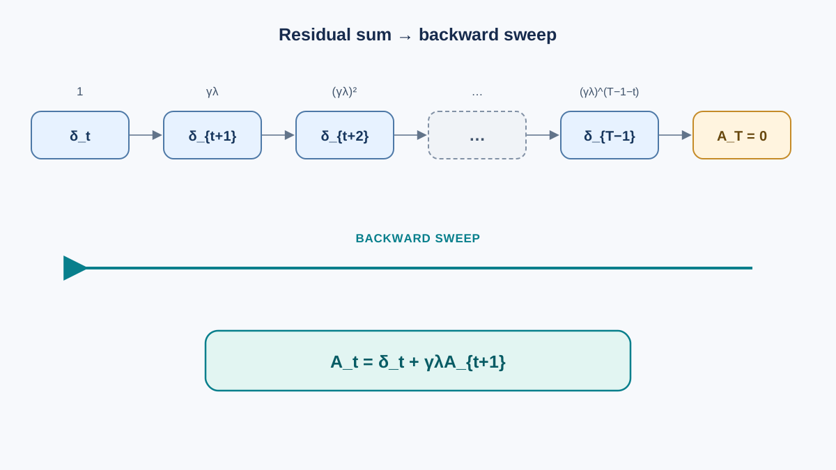
The infinite sum is not computable directly. Factor out the first term:

$\hat{A}_t^{\text{GAE}} = \delta_t + \gamma\lambda \sum_{l=0}^{\infty} (\gamma\lambda)^l \delta_{t+l+1} = \delta_t + \gamma\lambda \hat{A}_{t+1}^{\text{GAE}}.$

That is the recursion. Sweep backward over a batch of length $T$, initialize the tail advantage to zero, and you compute every advantage in $O(T)$ instead of $O(T^2)$:

advantages = np.zeros(T)
last_advantage = 0.0
for t in reversed(range(T)):
    delta = rewards[t] + gamma * values[t + 1] - values[t]
    last_advantage = delta + gamma * lam * last_advantage
    advantages[t] = last_advantage

The truncation is honest but biased. The infinite sum is cut at the batch boundary, and the tail advantage is replaced by zero. That is equivalent to assuming the critic is perfect beyond the horizon — which it is not.

Episode termination needs a mask. When an episode ends, the recursion must not bootstrap across the terminal state, because there is no next state to predict. Conflating termination with time-limit truncation corrupts the target: a time-limit cutoff is an artifact of the batch, not a property of the environment.

Here is a five-step worked example. Let $\gamma = 0.9$, $\lambda = 0.8$, so $\gamma\lambda = 0.72$. Rewards are $[1, 0, 2, 0, 1]$, and critic values are $[0.5, 0.6, 0.4, 0.8, 0.3, 0.0]$.

Sweep backward with $\hat{A}_5 = 0$:

• $\hat{A}_4 = 0.70 + 0.72 \cdot 0 = 0.70$
• $\hat{A}_3 = -0.53 + 0.72 \cdot 0.70 = -0.026$
• $\hat{A}_2 = 2.32 + 0.72 \cdot (-0.026) = 2.301$
• $\hat{A}_1 = -0.24 + 0.72 \cdot 2.301 = 1.417$
• $\hat{A}_0 = 1.04 + 0.72 \cdot 1.417 = 2.060$

Verify $\hat{A}_0$ against the sum: $1.04 + 0.72(-0.24) + 0.72^2(2.32) + 0.72^3(-0.53) + 0.72^4(0.70) = 1.04 - 0.173 + 1.203 - 0.198 + 0.188 = 2.060$. The recursion and the sum agree.

What the Critic's Error Does to the Estimator

Write the residual as the true residual plus the critic's error. Let $\epsilon_t = V_\phi(s_t) - V^\pi(s_t)$. Then

$\delta_t = \delta_t^{\text{true}} + \gamma \epsilon_{t+1} - \epsilon_t.$

Substitute into the GAE sum. The error terms accumulate under the same $(\gamma\lambda)^l$ weighting as the residuals:

$\hat{A}_t^{\text{GAE}} = \hat{A}_t^{\text{true}} + \sum_{l=0}^{\infty} (\gamma\lambda)^l (\gamma \epsilon_{t+l+1} - \epsilon_{t+l}).$

Lambda controls how far the critic's mistakes propagate into the advantage estimate. That is the real meaning of the parameter.

State the consequence plainly: lambda near 1 does not remove bias, it relocates it. The estimator stops trusting the critic and starts trusting the sampled trajectory. That trajectory is only unbiased if the samples come from the current policy — which is why off-policy reuse breaks the argument for large lambda.

Two failure modes follow:

• Lambda too low with an undertrained critic. The policy receives a systematically wrong signal. It learns slowly, or it learns the wrong thing, and the critic loss falling does not save you.
• Lambda too high with a badly undertrained critic. Advantage estimates become high-variance noise, and the policy gradient happily amplifies it. The run improves, then collapses.

Choosing Lambda: A Decision Rule Instead of a Default

Lambda around 0.95 is a common default because it keeps the effective horizon of the residual sum finite while retaining most of the Monte Carlo signal. The weights decay as $(\gamma\lambda)^l$, so the estimator effectively looks about $1/(1 - \gamma\lambda)$ steps ahead. With $\gamma = 0.99$ and $\lambda = 0.95$, that is roughly 100 steps.

Use the derivation as a diagnostic:

• Critic loss falling, policy not improving. Lambda is probably too low. The policy is being fed the critic's bias.
• Policy improving then collapsing. Lambda is probably too high. Advantage estimates are too noisy.
• Lambda = 0 reduces to one-step TD. Only sensible with a well-fit critic.
• Lambda = 1 is Monte Carlo. Only sensible with short episodes and an accurate policy sample.

One interaction that catches people: a short rollout truncates the sum earlier, so the same lambda behaves differently at different rollout lengths. If you change n_steps and keep lambda fixed, you changed the estimator.

Where the Derivation Stops Being Exact

The derivation assumes a fixed policy during the batch. Off-policy data or heavily reused batches break the unbiasedness argument for large lambda. It also treats $V$ as a function of state only; action-dependent critics and distributional critics require a different residual definition.

Most importantly: GAE is a variance-reduction device, not a correctness guarantee. It changes the variance of the gradient estimate, not the direction the gradient points in expectation. If the advantage is biased, GAE does not fix it — it redistributes the bias across the horizon.

Here is your next move. Instrument a training run to log the mean absolute TD residual alongside the policy loss. Sweep lambda across a few values and watch how the two move together. When the residual is large and lambda is low, the policy is learning from a critic that does not know what it is talking about. When the residual is small and lambda is high, you are paying variance for a signal you already had. The math becomes something you can observe rather than something you memorized.