
Deriving the Policy Gradient: From Expected Return to a Practical Estimator
The REINFORCE update looks like a magic trick: multiply a log-probability by a return, add it to the parameters, and hope the policy improves. It is not a…

Key topics
The REINFORCE update looks like a magic trick: multiply a log-probability by a return, add it to the parameters, and hope the policy improves. It is not a trick. It is what falls out when you differentiate an expectation you cannot differentiate directly.
If you already understand why stochastic policies matter and how sampled outcomes push action probabilities around, this article fills in the missing middle. We take the expected-return objective, differentiate it honestly, and arrive at the estimator you actually compute. The point is not to recite a formula. The point is to make every term in the update do a job you can name.
Why You Cannot Just Differentiate the Return
Start with the target. We want to maximize the expected return of a parameterized policy:
Here is the parameter vector, is a trajectory, and is its return. The expectation runs over trajectories sampled by executing the policy in the environment.
The obstacle is structural. The parameter sits inside the distribution you are averaging over, not inside the return. The environment decides rewards and transitions; it has no idea exists. Differentiate a sampled return with respect to and you get zero. The reward did not change because you nudged a weight in your network. The trajectory did.
You also never observe directly. You observe sampled trajectories and their returns. Any usable gradient must therefore be expressible as an expectation itself, so a sample mean can estimate it. That is the whole game: turn the gradient of an expectation into an expectation of something computable.
Notation: Policy, Trajectory, Return, Objective
Before the algebra, fix the symbols.
The policy is a distribution over actions given a state, parameterized by . It is the only object we control. Everything else — the environment's dynamics, the reward function, the initial state distribution — is fixed and independent of .
A trajectory is a sequence of states and actions. Its probability factors into three kinds of terms:
The initial-state term and the transition term belong to the environment. Only the policy terms carry .
The return is the sum of rewards along the trajectory. Two conventions are common: finite-horizon undiscounted, , and infinite-horizon discounted, . The derivation is nearly identical for both. I use the finite-horizon form to keep the notation light and note where discounting would slot in.
The objective is , and we want .
Knowledge check
Check your understanding
Answer this question before you continue.
The Log-Derivative Trick, Step by Step
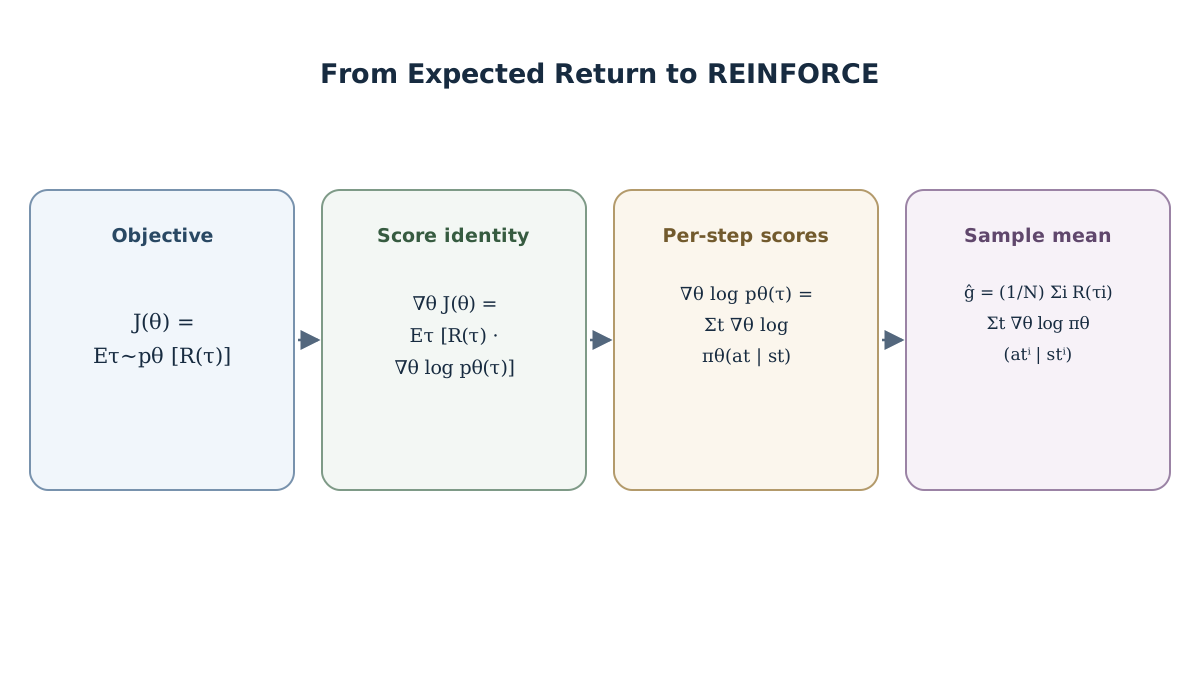
Write the expectation as a sum over trajectories:
Push the gradient inside the sum. The return does not depend on , so it passes through untouched:
Now the useful move. Multiply and divide by :
The fraction is the score function. Apply the identity with :
Collapse the sum back into an expectation:
This is the likelihood-ratio form, and it is the hinge of the entire derivation. The gradient is now an expectation of something you can compute from sampled trajectories. The probability density has been converted into a log-probability gradient, which is far easier to work with.
Knowledge check
Check your understanding
Answer this question before you continue.
From Trajectory Probability to Per-Step Log-Probabilities
The expression above is still about whole trajectories. To make it implementable, decompose the log-probability.
Take the log of the trajectory probability:
Differentiate with respect to . The initial-state term and every transition term are environment functions with no dependence, so their gradients are zero. Only the policy terms survive:
Substitute this back:
This is where the derivation stops being about trajectories and starts being about individual state-action pairs. The environment terms dropped out because they carry no parameter dependence. What remains is a sum of per-step log-probability gradients, each weighted by the return of the trajectory it came from.
Knowledge check
Check your understanding
Answer this question before you continue.
The Estimator You Actually Compute
Replace the expectation with a sample mean over collected trajectories:
This is the REINFORCE estimator. It is unbiased: its expectation equals the true policy gradient. It is also high variance, and the reasons are worth naming.
Three assumptions are baked in:
- The policy is differentiable in . If you cannot take , the estimator does not exist.
- Actions are sampled from the current policy. This is an on-policy estimator. Reusing data from an older policy requires importance sampling, which changes the estimator.
- Enough trajectories are collected for the sample mean to be meaningful. A single trajectory gives a noisy, possibly misleading estimate.
The variance problem has a specific shape. The raw return weights every action in the trajectory equally, including actions taken long before the reward arrived. An action that happened to precede a lucky reward gets credit it did not earn. Two standard refinements address this without changing the expectation:
Reward-to-go replaces with the sum of rewards from timestep onward. Actions before a reward no longer receive credit for it. The estimator stays unbiased because the discarded terms have zero expectation under the policy.
Baselines subtract a state-dependent value from the return weight. Any baseline that does not depend on the action leaves the expectation unchanged, but a good baseline — typically a learned value function — reduces variance substantially. This is the seed of actor-critic methods, though the full machinery is a separate topic.
Worked Example: Reading the Update
Make it concrete. Suppose a single state with two actions, and . The policy is a softmax over two logits, and the current probabilities are and .
For a softmax policy, the score points in the parameter-space direction that increases the probability of the sampled action and decreases the others. The return scales that direction. Both facts are local to the current parameters and the sampled action — they describe one gradient-ascent contribution, not a global law about how the policy will move after many updates.
Now sample. Suppose the agent takes and receives a return of . The update adds a positive multiple of the score for , so this single contribution pushes upward. Suppose instead the agent takes and receives a return of . The update subtracts, and this contribution pushes downward.
| Sampled action | Return | Local effect on |
|---|---|---|
| Pushes up | ||
| Pushes down | ||
| Nearly unchanged |
The third row is the quiet one. When the return is near zero, the update nearly vanishes. This is why sparse-reward problems learn slowly: most sampled trajectories carry almost no signal, and the gradient has almost nothing to scale.
Two qualifications matter here, because they are easy to overread.
First, the sign of a raw return is only meaningful relative to the reward origin. A return of is not automatically "good" if the environment hands out for doing nothing. What the update actually reinforces is the sampled action relative to the other actions the policy could have taken — and that relative comparison is what a baseline or advantage estimate makes explicit. With an uncentered return, the sign is a statement about the reward scale, not a verdict on action quality.
Second, with shared parameters across states and actions, a single update does not move only the sampled action's probability. The score for one state-action pair is a direction in the full parameter vector, and that direction can shift probabilities elsewhere. The clean two-logit picture is a teaching device, not a promise about every network.
The single most useful thing to carry away: the score supplies the direction; the return supplies the weight. The policy does not learn what to do from the return. It learns how much to reinforce what it already sampled.
Knowledge check
Check your understanding
Answer this question before you continue.
Where the Derivation Stops Being Exact
The derivation is clean, but its assumptions have edges.
It assumes a stochastic, differentiable policy. Deterministic policies need a different route, because the log-probability of a deterministic action is not a well-behaved function of .
It assumes on-policy sampling. The moment you reuse trajectories from an older policy, the expectation is over the wrong distribution, and you need importance sampling to correct it. That correction is not free — it adds its own variance.
The unbiasedness claim is about the expectation, not about any single batch. A high-variance estimator can produce individual updates that point the wrong way. A correct gradient in expectation is not a correct gradient on your one noisy batch.
Finally, the derivation says nothing about step size. A perfectly computed gradient can still produce a destructive update if the learning rate is too large. The gradient tells you the direction of steepest ascent locally; it does not tell you how far to walk.
What to Do With This
When you see a policy-gradient update in code or a paper, read it in two parts. First, find the log-probability term — that is the direction, and it points toward increasing the probability of what was sampled. Second, find the return or advantage term — that is the weight, and it decides whether the direction is reinforced or reversed.
Then check the sampling assumption. Is the implementation on-policy? Does it reuse old data? If so, where does the importance-sampling correction appear?
The natural next step is to implement the estimator on a small environment — a two-action bandit or a tiny gridworld — and watch the action probabilities move after each update. Print the log-probability, the return, and the resulting parameter change. The formula stops being abstract the moment you see a positive return nudge a probability upward and a negative return pull it back down.
Once that runs, variance reduction is the next topic worth your time. Reward-to-go and baselines are the first tools, and they are where the gap between the textbook estimator and a usable one starts to close.
Knowledge check
Final check
Finish the article by checking the ideas you just learned.
References
Build a stronger RL mental model
Use structured resources to connect equations, algorithms, and observable agent behavior.


