
Implement Options as Temporally Extended Actions in a Small RL Task
You have read that options compress repeated action sequences into single decisions. Then you sit down to code one, and the boundary dissolves: where does…

Key topics
You have read that options compress repeated action sequences into single decisions. Then you sit down to code one, and the boundary dissolves: where does the option end and the environment begin?
Here is the model that fixes it. An option is a triple — an initiation set, an internal policy, and a termination rule — that the agent consults at decision time. The environment never sees any of that. It only ever receives primitive actions. Once you hold that boundary in your head, the code almost writes itself.
By the end of this tutorial you will have one runnable script that mixes primitive actions with a single option, prints option duration, decision-step counts, and accumulated return, and shows all three numbers move when you change one line of the termination rule.
What You Are Actually Building
The deliverable is a single Python file. It runs a small deterministic tabular task, executes an option alongside primitive actions, and prints a comparison table across a primitives-only baseline and two termination rules.
I am assuming two things are already in place:
- You have a tiny deterministic tabular environment with verified transitions, rewards, and terminal behavior. If not, build and smoke-test that first — this article does not rebuild it.
- You have read the conceptual explanation of options and know the triple: initiation set I, internal policy π, termination condition β.
Everything here is plain Python. No RL library, no Gym, no neural network. I use Python 3.10+ syntax, but nothing exotic. The task is tabular and deterministic, so every number you print is reproducible — run it twice, get the same output.
Why tabular first? Because with a small state space you can print the entire option trace and watch the mechanism move. With a loss curve, you would be inferring the mechanism from a squiggle. Print the trace. Read the states. Then trust the abstraction.
Representing an Option as Three Callables
An option is not a macro that runs some actions. It is a small object holding three functions, each answering one question at runtime.
from dataclasses import dataclass
from typing import Callable

@dataclass
class Option:
    initiation: Callable[[int], bool]          # can this option start here?
    policy: Callable[[int], int]               # what primitive action to take?
    termination: Callable[[int, int], bool]    # stop now?
    name: str = "option"
Three design choices deserve a sentence each.
The internal policy returns a primitive action, not another option. Keep the first implementation flat. If your option's policy could return another option, you have just built a hierarchy of hierarchies, and the environment interface gets complicated for no gain yet. Flat first.
Termination takes the step count as well as the state. Some termination rules are state-based ("stop when you reach the corridor"), some are budget-based ("stop after four steps"). The signature termination(state, steps_taken) allows both without a rewrite when you switch variants later.
Initiation is a predicate, not a hardcoded list. A predicate makes the "where can this option start" question explicit and testable. You can call option.initiation(s) for any state and get a yes or no. A list hides that question inside membership checks scattered through your code.
Note: This is a hand-specified option. You are writing the internal policy yourself. Learning option policies is a separate problem and out of scope here. You are testing the mechanism, not the learning of it.
Knowledge check
Check your understanding
Answer this question before you continue.
Wiring the Option Into the Decision Loop
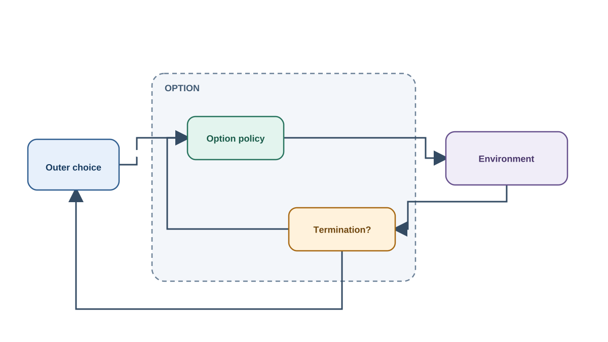
Here is the smallest integration that actually runs. The environment is a one-dimensional corridor of 8 states, 0 through 7. State 0 is the start, state 7 is the goal, and the primitive actions are LEFT and RIGHT. Stepping off either end keeps you in place. Reaching state 7 ends the episode with reward +1; every other step gives -0.01.
N_STATES = 8
GOAL = 7
LEFT, RIGHT = 0, 1

def step(state, action):
    if state == GOAL:
        return state, 0.0, True
    nxt = max(0, min(N_STATES - 1, state + (1 if action == RIGHT else -1)))
    done = nxt == GOAL
    return nxt, (1.0 if done else -0.01), done
Now the option. Its job: walk right until it reaches the goal, or until a step budget runs out.
def make_option(termination):
    return Option(
        initiation=lambda s: s < GOAL,
        policy=lambda s: RIGHT,
        termination=termination,
        name="walk-right",
    )
The decision loop is where the abstraction lives. At each decision point, filter options by initiation, pick one, then execute its internal policy until termination fires. The environment steps happen inside that execution.
def run_episode(option=None, use_option=True):
    state = 0
    total_reward = 0.0
    env_steps = 0
    decision_steps = 0
    option_durations = []

    while state != GOAL:
        decision_steps += 1
        if use_option and option.initiation(state):
            steps_taken = 0
            while True:
                action = option.policy(state)
                state, r, done = step(state, action)
                total_reward += r
                env_steps += 1
                steps_taken += 1
                if done or option.termination(state, steps_taken):
                    break
            option_durations.append(steps_taken)
        else:
            state, r, done = step(state, RIGHT)
            total_reward += r
            env_steps += 1

    return total_reward, env_steps, decision_steps, option_durations
Read the inner loop carefully. The option does not skip time. It decides what to do during time. Every environment step still happens, one at a time, and reward still accumulates one step at a time. The only thing the option changes is how many of those steps happen between two decisions.
That is the whole point of temporal abstraction, and it is why decision-step count and environment-step count diverge. In the primitives-only run, they are equal. With the option active, decision steps drop while environment steps stay roughly the same. If those two numbers are identical when the option is on, your option is not extending anything — check the termination rule first.
Knowledge check
Check your understanding
Answer this question before you continue.
Reading the Numbers: Duration, Decision Steps, Returns
Three metrics tell you whether the option is doing real work.
Option duration is the number of environment steps consumed per option invocation. A duration of 1 means the option is behaving like a primitive action and your termination rule is too aggressive.
Decision-step count per episode should drop when the option covers ground that primitives would have covered one step at a time. This is the compression you are buying.
Accumulated return only means something against a baseline. Run the primitives-only version first, then compare. An absolute number in isolation tells you nothing.
Here is the comparison harness. It runs the primitives-only baseline and both termination rules — one state-based, one budget-based — through the same measurement path:
def terminate_at_goal(state, steps_taken):
    return state == GOAL

def terminate_after_budget(state, steps_taken):
    return steps_taken >= 4

runs = [("primitives only", None, False)]
for label, term in [("goal", terminate_at_goal), ("budget-4", terminate_after_budget)]:
    runs.append((label, make_option(term), True))

for label, opt, use_opt in runs:
    r, es, ds, durs = run_episode(opt, use_option=use_opt)
    mean_dur = sum(durs) / len(durs) if durs else 0
    print(f"{label:15s} return={r:+.2f} env_steps={es} decisions={ds} mean_dur={mean_dur:.1f}")
On the 8-state corridor, the output looks like this:
| Run | Return | Env steps | Decision steps | Mean duration |
|---|---|---|---|---|
| primitives only | +0.93 | 7 | 7 | — |
| goal | +0.93 | 7 | 1 | 7.0 |
| budget-4 | +0.93 | 7 | 2 | 3.5 |
The return is identical across all three because the corridor is trivial and the option always walks right. The interesting column is decision steps: 7, then 1, then 2. The goal-terminated option compresses the whole episode into a single decision. The budget-terminated option needs two decisions because it runs out of budget mid-corridor and gets re-invoked.
Common mistake: Treating a shorter episode as automatically better. It is not. Check whether the option is actually reaching useful states or just terminating early and forcing the outer loop to re-decide. Duration and decision steps together tell you which one happened.
Knowledge check
Check your understanding
Answer this question before you continue.
Changing the Termination Rule and Watching What Moves
This is the experiment the whole article builds toward. Before you run it, predict the outcome.
Variant A — goal-directed termination. The option runs until it reaches the goal state. You should expect long durations and very few decision steps. The option commits to a plan and follows it to the end.
Variant B — budget termination. The option runs for a fixed number of steps regardless of state. You should expect shorter durations and more decision steps, because the option gets cut off before it finishes and the agent has to re-invoke it.
Now run both and compare against your prediction. The gap between what you expected and what printed is the actual lesson. In the corridor above, the gap is small because the task is trivial. Make the corridor longer — 20 states, say — and the budget option starts needing five decisions where the goal option needs one.
The decision rule to carry forward: a termination rule is a bet about how long a useful sub-behavior stays useful. Terminate too early and you pay decision overhead on every re-invocation. Terminate too late and you commit to a stale plan when the situation has already changed underneath you. There is no universally correct rule — only a rule that matches how long your sub-behavior actually stays relevant.
Failure Modes You Will Hit First
Debug by symptom, not by guesswork.
Option never terminates. Duration explodes, the episode stalls, and the return flatlines. Usually the termination predicate can never be satisfied from the states where the option starts. Print the state and step count inside the inner loop and watch whether the termination condition ever evaluates true.
Option terminates immediately. Duration is 1 everywhere and the option adds overhead without changing behavior. Usually the initiation set overlaps states the termination rule already excludes — the option starts in a state where it instantly ends.
Initiation set and termination rule contradict each other. The option can start in a state where it instantly ends. This is legal but almost always a design error. Test it directly: for every state where initiation(s) is true, check whether termination(s, 0) is also true. If so, that state is a dead entry point.
Reward double-counting. If you accumulate reward both inside the option and in the outer loop, returns inflate. Decide once where reward is recorded. In the code above, reward is recorded inside the inner loop only, and the outer loop never touches it.
Off-by-one in step counting. Whether the terminating step belongs to the option or to the next decision point changes every duration number you print. Pick a convention, write it in a comment, and stick to it. I count the terminating step as part of the option, which is why the goal-terminated option shows a duration of 7 rather than 6.
Knowledge check
Check your understanding
Answer this question before you continue.
Where This Leads Next
You now own a working option implementation, a comparison harness, and a decision rule for termination design. That is real progress — you have turned an abstract triple into code that runs and prints numbers you can argue with.
The honest limitation: this option was hand-specified. You tested the mechanism, not the learning of it. The next question worth asking is what changes when the internal policy is learned rather than written by hand. That shift turns a bookkeeping problem into a credit-assignment problem, because now the option's policy has to figure out which of its internal actions earned the reward at termination.
Your concrete next action: add a second option with a different initiation set — say, one that walks left from the right half of the corridor — and check whether the two options ever compete at the same decision point. When they do, you have to choose between them, and that choice is where hierarchical control actually begins.
Knowledge check
Final check
Finish the article by checking the ideas you just learned.
Build a stronger RL mental model
Use structured resources to connect equations, algorithms, and observable agent behavior.


