
Options in Reinforcement Learning: How Temporally Extended Actions Work
A flat policy re-decides everything, every step. Options let it decide once and commit.

Key topics
A flat policy re-decides everything, every step. Options let it decide once and commit.
Why Long Horizons Break Flat Policies
Watch an agent that has learned a clean policy for a short task fail on a long one. The network is large enough. The reward signal is well-shaped. The training loop is the same one that worked before. Yet the agent drifts: it takes the right first step, the right second step, and somewhere around step forty it is doing something that no longer resembles the routine you designed.
The usual diagnosis is "not enough training." That diagnosis is usually wrong. The problem is not decision quality. It is decision granularity.
A flat policy makes a fresh choice at every primitive step. Over a 200-step routine, that is 200 separate decision points, each with its own chance to be slightly wrong. Small per-step errors do not stay small; they compound into trajectory drift, and the state distribution the agent visits slowly slides away from the one it was trained on. Meanwhile, exploration has to find a coherent 200-step sequence by sampling primitive actions, which is a search problem whose useful region shrinks sharply as the horizon grows.
You already know from earlier work that delayed reward makes credit assignment hard and that horizons define what a return even means. The point here is narrower and more actionable: the number of distinct decision points an agent must get right scales with horizon length, and that combinatorial cost is what breaks the flat policy. The fix is not to make each decision better. It is to make fewer, longer decisions, each carrying a coherent sub-behavior.
That is what temporally extended actions buy you.
Knowledge check
Check your understanding
Answer this question before you continue.
What an Option Actually Is
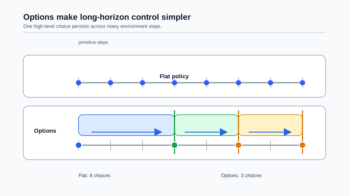
An option is a closed-loop policy that runs for a while. Formally, it is a triple:
- Initiation set $I_\omega$: the states where the option is allowed to start.
- Internal policy $\pi_\omega$: the distribution over primitive actions the option emits while it is running.
- Termination condition $\beta_\omega(s)$: the probability that the option stops in state $s$.
The termination condition is a probability, not a hard rule. That single design choice is what makes the framework general — and what makes it dangerous, as we will see.
The cleanest way to hold this in your head is to notice that a primitive action is just a degenerate option. Its internal policy puts all probability on one action, and its termination condition is 1 everywhere: it always ends immediately. Options generalize the action set: you are not replacing the MDP, you are enriching its action vocabulary.
Above the options sits a second decision maker: the policy over options $\mu$. It selects an option, then waits. It does not re-decide at every primitive step. It re-decides only when the running option terminates.
Picture a timeline. Primitive steps are ticks. An option is a bracket spanning several ticks. The policy over options makes a choice at each bracket boundary and nowhere in between. That is the whole mechanism: one decision, many steps, one commitment.
Common mistake: Treating the option's internal policy as fixed. It is a policy — it can be stochastic, learned, and state-dependent. An option is not a script; it is a small controller.
Knowledge check
Check your understanding
Answer this question before you continue.
How Options Change the Bellman Structure
Here is where the abstraction touches machinery you already have. Options do not replace Bellman reasoning. They re-index it.
Define the option-value function $Q_\Omega(s, \omega)$: the expected discounted return of being in state $s$, committing to option $\omega$, and thereafter following the policy over options. The backup for this quantity is a multi-step version of the one-step backup you already know.
The cleanest way to see it is to separate the two cases at the moment the option ends. Suppose the option runs from state $s$ for some number of primitive steps, accumulating discounted reward $R$ along the way, and finally terminates in state $s'$. Then the option value satisfies:
$$ Q_\Omega(s, \omega) = \mathbb{E}\left[ R + \gamma^{\tau} , V_\Omega(s') \right] $$
where $\tau$ is the (random) number of primitive steps the option took, $R$ is the discounted reward accumulated during those steps, and $V_\Omega(s') = \mathbb{E}{\omega' \sim \mu(\cdot \mid s')}\left[ Q\Omega(s', \omega') \right]$ is the value of the state under the policy over options.
Read it as three pieces. First, reward accumulates while the option runs — that is $R$. Second, the discount factor is raised to the option's duration $\tau$, because the option consumed $\tau$ primitive steps, not one. Third, when the option terminates, control returns to the policy over options, which picks the next option according to $\mu$.
The termination function appears explicitly in the backup. It decides how much weight goes to continuing versus switching, and it shapes the distribution of $\tau$. This is why termination design is not cosmetic: it is a term in the value equation, and a badly chosen $\beta$ corrupts the value estimate the top-level policy learns from.
Note: The equation above is the fixed-policy version, where continuation after termination follows $\mu$. If you are doing option-level control — improving the policy over options — you replace $V_\Omega(s')$ with $\max_{\omega'} Q_\Omega(s', \omega')$. The two cases are not interchangeable; mixing them silently is a common source of bugs.
The underlying object is a semi-Markov decision process. Primitive steps still generate rewards and state transitions. But one option execution produces a single variable-duration high-level transition: from the option's start state to its termination state, carrying the accumulated discounted return and the duration $\tau$. The higher-level backup uses that coarser transition. Same fixed-point reasoning, coarser decision clock. The convergence story is the same story you already trust for ordinary Bellman backups — do not re-derive it here. What changes is the unit of decision, not the mathematics of value.
A useful mental image: a two-level tree. The top level branches over options. Each branch expands downward into a short chain of primitive steps. The top level never sees the individual steps; it only sees where each chain ends and how much reward it carried.
Knowledge check
Check your understanding
Answer this question before you continue.
Designing Initiation Sets and Termination Conditions
This is where most option implementations succeed or fail, so treat both as first-class design decisions.
Initiation sets control availability. An option available everywhere is trivial to specify — and it lets the policy over options pick a skill in a state where that skill cannot possibly succeed. A tight initiation set is a promise: this option is only offered where it has a chance. The cost is that you now have to know where that is.
Termination conditions control commitment length. This is the sharper knife. Terminate too early and you have rebuilt a primitive action with extra bookkeeping. Terminate too late and the option overstays, burning steps and blocking better choices. The termination condition is the dial that sets how much temporal abstraction you actually get.
There are two broad strategies, and they trade off cleanly:
| Approach | How termination is set | Strength | Cost |
|---|---|---|---|
| Hand-specified | Subgoals, pseudo-rewards, fixed termination regions | Interpretable, reusable, inspectable | Requires domain knowledge; does not adapt |
| Learned | Termination function learned jointly with the policy | No subgoal specification burden | Options are hard to name, hard to reuse, tied to training config |
Learned termination — the option-critic style of approach — removes the burden of telling the system where each skill should end. That is a real win. It also produces options you cannot easily describe, cannot lift into a new task, and cannot debug by inspection. The abstraction works; the legibility is gone.
Practical rule: If you cannot state in one sentence what an option is for, its termination condition is probably not doing useful work.
Knowledge check
Check your understanding
Answer this question before you continue.
Benefits, Costs, and Failure Modes
Options are a bet. Here is what you are betting on, and what you are risking.
The benefits. Fewer high-level decisions per episode means a shorter effective horizon for the top-level policy to reason over, which can improve sample efficiency on long-horizon tasks. And a well-designed option is reusable: a sub-behavior that solves "navigate to the door" can be lifted into a new task that shares that sub-behavior, without retraining from scratch.
The costs. The option set is a new design surface. A bad option library is worse than no abstraction at all, because it constrains what the top-level policy can express. You have added a layer, and that layer can lie to you.
The failure modes are worth naming precisely, because each one has a distinct signature:
- Degenerate options. They terminate almost immediately, collapsing back to primitive control while adding overhead. You paid for abstraction and got bookkeeping.
- Runaway options. They never terminate. The top-level policy is starved of decisions, and the agent can loop indefinitely inside a single skill.
- Illegible learned options. Without subgoals, learned options generalize poorly and cannot be transferred or inspected. You have a policy you cannot reason about.
When not to use options. Short-horizon tasks do not need them. Tasks where the useful sub-behaviors are unknown and cannot be discovered cheaply will produce garbage options. And if a flat policy already trains reliably, adding options is ceremony. The honest starting point is flat; earn the abstraction.
A Small Experiment to Feel the Tradeoff
You do not need a full hierarchical RL system to see this mechanism move. You need a gridworld and a log.
Take a small multi-room gridworld. Hand-write two or three options with explicit initiation sets and termination regions — for example, "go to the north door" and "go to the east door." Then run the same environment twice: once with a flat policy, once with the option-augmented policy.
Hold everything else fixed: same environment, same reward, same training budget, same evaluation episodes. Then log four things per run:
- Task performance: success rate and primitive steps-to-goal.
- Option-selection count: how many times the top-level policy made a decision.
- Option duration distribution: how long each option ran before terminating.
- Termination locations: where in the state space each option ended.
The comparison that matters is not the headline number. It is the termination histogram. That histogram is the fastest diagnostic you will build:
- A spike at length 1 means degenerate options. Your abstraction is a no-op.
- A long tail with no termination means runaway options. Your top-level policy is asleep.
- A clean distribution around a few steps means the option is doing real work.
One caveat: if you hand-code the options, this experiment tests execution and coordination, not skill discovery. The options already know the route; the question is whether the top-level policy can use them. That is still a useful test — but do not read it as evidence that the system learned anything about the task structure.
I would build that instrumentation before tuning anything else. The histogram tells you whether the abstraction is earning its keep, and it tells you in one run.
The Decision Rule
Options are a bet that your task contains reusable sub-behaviors and that you can name where each one starts and stops. If you can write those two conditions down — the initiation set and the termination condition — the abstraction pays for itself. If you cannot, a flat policy is the honest starting point, and no amount of extra training will substitute for the missing structure.
Learning termination is a later step, not a default one. It becomes the right move when hand-designed boundaries are the demonstrated bottleneck: your options are useful, your histogram shows they run for sensible durations, but the fixed termination points are consistently mistimed and you have run out of patience for tuning them by hand. If interpretability, safety, or transfer matter more than that convenience, keep the boundaries hand-specified and accept the tuning cost.
Before you go there, build the option-length histogram. It is the instrument that will tell you whether learned termination is doing anything at all — or just quietly collapsing your hierarchy back into a flat policy wearing a costume.
Knowledge check
Final check
Finish the article by checking the ideas you just learned.
References
Research updated Sep 9, 2026


