Deriving Semi-Markov Bellman Equations for Options

An option that runs for five steps collects five rewards. The primitive Bellman backup discounts one. That single mismatch is the whole reason the semi-Markov backup exists.

If you already know what options are and how the one-step Bellman backup is derived, the next question is mechanical: what changes when the decision unit is a policy that runs for a random number of steps? The answer is not a cosmetic tweak. The reward term becomes an accumulated sum, the continuation discount becomes a random exponent, and the model becomes a joint distribution over next state and transit time. Let's derive each piece.

Why the One-Step Backup Breaks for Options

The primitive backup for a policy π is:

$V^\pi(s) = \sum_a \pi(a \mid s) \left[ r(s,a) + \gamma \sum_{s'} p(s' \mid s,a)\, V^\pi(s') \right]$

Read it as: expected immediate reward plus the discounted value of the successor state. Two assumptions are baked in. The transition consumes exactly one time step. The reward is a single scalar, not a sum over a trajectory.

Both assumptions fail the moment you substitute an option $o = \langle \mathcal{I}, \pi_o, \beta \rangle$ for a primitive action. Suppose the option's internal policy runs for $k$ steps before its termination condition $\beta$ fires. It collects rewards $r_{t+1}, r_{t+2}, \dots, r_{t+k}$. The naive substitution credits one reward and applies $\gamma$ once. You undercount the reward stream and you undercount the elapsed time. The discount on the continuation term should be $\gamma^k$, not $\gamma$, and $k$ is a random variable.

The repair is to describe the option's outcome with a joint distribution over three things: the terminal state $s'$, the accumulated discounted reward $r$ collected along the way, and the duration $k$. Once that distribution exists, the backup can be written cleanly.

Notation and Assumptions

Before the derivation, pin down every symbol.

An option is a triple $o = \langle \mathcal{I}, \pi_o, \beta \rangle$: an initiation set $\mathcal{I} \subseteq \mathcal{S}$, an internal policy $\pi_o$, and a termination condition $\beta$. The internal policy is what generates the intermediate rewards — it is not a single action but a distribution over actions at each internal step.

When option $o$ is initiated in state $s$, three random variables describe its outcome:

• $s'$ — the state in which the option terminates
• $r$ — the cumulative discounted reward collected during execution, $r = \sum_{j=1}^{k} \gamma^{j-1} r_{t+j}$
• $k$ — the number of time steps between initiation and termination

The option model is the joint distribution over next state and transit time, $p(s', k \mid s, o)$. From it, define the discounted transition probability:

$p^o_{ss'} = \sum_{k=1}^{\infty} \gamma^k \, p(s', k \mid s, o) = \mathbb{E}\!\left[\gamma^k \mathbb{1}\{s_{t+k} = s'\} \mid \mathcal{E}(o,s)\right]$

This folds the discount into the state prediction so the backup can be written as a single sum. The expected cumulative reward is $r^o_s = \mathbb{E}[r \mid \mathcal{E}(o,s)]$, where $\mathcal{E}(o,s)$ denotes the event of initiating $o$ in $s$.

Three assumptions make this valid. Time is discrete. The option's policy and termination condition are stationary. And the semi-Markov property holds: the outcome depends only on the initiating state and the option, not on the history before initiation.

Warning: History-dependent termination conditions — timeouts, or $\beta$ that depends on the trajectory so far — break the state-only form. You then need a history-indexed value function $Q^\mu(h, o)$, and the compact backup below no longer applies.

Deriving the Option Value Backup

Start from the return, conditioned on initiating $o$ in $s$:

$Q^\mu(s, o) = \mathbb{E}\!\left[ r_{t+1} + \gamma r_{t+2} + \cdots + \gamma^{k-1} r_{t+k} + \gamma^k V^\mu(s_{t+k}) \;\middle|\; \mathcal{E}(o,s) \right]$

The first $k$ terms are the within-option reward stream. The last term is the continuation. Notice that $k$ appears in the exponent of the continuation discount and as the upper limit of the reward sum — it is a random variable living inside the expectation.

Group the reward stream into $r$ and apply the tower property by conditioning on the option's outcome $(s', k)$:

$Q^\mu(s, o) = \mathbb{E}\!\left[ r + \gamma^k V^\mu(s') \;\middle|\; \mathcal{E}(o,s) \right]$

Now substitute the definition of $V^\mu(s')$ — the value of the state under the policy over options $\mu$:

$V^\mu(s') = \sum_{o' \in \mathcal{O}_{s'}} \mu(s', o')\, Q^\mu(s', o')$

This closes the recursion. Expanding the expectation over the joint distribution gives the summed form:

$Q^\mu(s, o) = r^o_s + \sum_{s'} p^o_{ss'} \sum_{o' \in \mathcal{O}_{s'}} \mu(s', o')\, Q^\mu(s', o')$

And the state-value backup follows by marginalizing over the option choice:

$V^\mu(s) = \sum_{o \in \mathcal{O}_s} \mu(s, o) \left[ r^o_s + \sum_{s'} p^o_{ss'}\, V^\mu(s') \right]$

The action-value version comes from the same route, replacing $V^\mu(s')$ with the max over options for the optimality variant. One identity is worth keeping: $Q^\mu(s, o) = V^{o\mu}(s)$ — the option value at a state equals the state value under the flat policy that the option induces. That identity is what lets you move between the two views without re-deriving anything.

Where the Discount Exponent Comes From

The continuation term carries $\gamma^k$, and $k$ is random. That means the effective discount applied to the successor value is $\mathbb{E}[\gamma^k]$, not $\gamma$. Since $0 < \gamma < 1$, $\mathbb{E}[\gamma^k] < \gamma$ whenever the option can last more than one step. The gap widens as the option's expected duration grows.

This is a real effect, but it is narrower than it first looks. The duration discount lowers the continuation contribution — the discounted value of whatever state the option hands off to. It does not by itself make a longer option worse overall. A longer option also accumulates more within-option reward, and it may terminate in a better state. Those two effects can easily outweigh the extra discounting and reverse the ranking.

So the honest statement is conditional: hold the terminal-state distribution and the continuation values fixed, and a longer duration lowers the continuation term. Change the rewards or the terminal states and the comparison can flip. If you want to see this, take the worked example below and raise the slow outcome's cumulative reward from 1.5 to 2.5. The slow option now wins despite paying $\gamma^2$ instead of $\gamma^1$.

The discounted transition probability $p^o_{ss'}$ is exactly this discount folded into the state prediction. That is why the compact backup has no visible $\gamma$ in the continuation term: the discount has been absorbed into the model. When you estimate $p^o_{ss'}$ from data, you are estimating a quantity that already contains the duration-weighted discount, which is why duration estimation error propagates directly into the value.

Worked Example: A Two-Step Option Backup

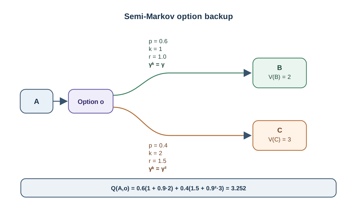
Take a three-state environment $\{A, B, C\}$ with $\gamma = 0.9$. One option $o$ is initiated in $A$. Its internal policy and termination condition produce two possible outcomes:

The cumulative reward for the slow case already includes the discount on the second reward: $r = r_{t+1} + \gamma r_{t+2}$.

Compute the expected cumulative reward:

$r^o_A = 0.6(1.0) + 0.4(1.5) = 0.6 + 0.6 = 1.2$

Compute the discounted transition probabilities:

$p^o_{AB} = 0.6 \cdot \gamma^1 = 0.6 \cdot 0.9 = 0.54$ $p^o_{AC} = 0.4 \cdot \gamma^2 = 0.4 \cdot 0.81 = 0.324$

Note that $p^o_{AB} + p^o_{AC} = 0.864 < 1$. The mass that "disappeared" is the duration discount — it is not a probability leak, it is the discount doing its job.

Now suppose $V^\mu(B) = 2.0$ and $V^\mu(C) = 3.0$. The backup gives:

$Q^\mu(A, o) = 1.2 + 0.54(2.0) + 0.324(3.0) = 1.2 + 1.08 + 0.972 = 3.252$

Compare against the naive one-step substitution, which would treat $o$ as a single action with expected reward 1.2 and a plain transition to a blended successor:

$Q_{\text{naive}} = 1.2 + 0.9\big[0.6(2.0) + 0.4(3.0)\big] = 1.2 + 0.9(2.4) = 3.36$

The naive backup overestimates by about 0.11. The error is small here because the durations are short and $\gamma$ is close to 1, but the direction is consistent for this outcome distribution: the naive version under-discounts the continuation, so it overvalues the option relative to the correct backup. The error grows with duration and with the gap between the two successor values.

Common mistake: Reading the 0.11 gap as a general rule that "longer options are worse." The gap here is a comparison between two backups of the same option, not a comparison between two different options. Ranking options requires comparing their full $r^o_s + \sum_{s'} p^o_{ss'} V^\mu(s')$ values, not their durations.

Primitive Backup vs Option Backup

The reduction check matters: when the option always terminates in one step, $k = 1$ deterministically, $p^o_{ss'} = \gamma\, p(s' \mid s, o)$, and the option backup collapses exactly to the primitive backup. If your derivation does not pass this check, something is wrong.

When the Semi-Markov Backup Applies and When It Does Not

The backup is valid when options are treated as opaque, indivisible units and their outcomes depend only on the initiating state and the option. That is the semi-Markov property, and it is the load-bearing assumption.

It breaks in three places. History-dependent termination — timeouts, or $\beta$ that inspects the trajectory — requires a history-indexed value function. A non-stationary option policy invalidates the fixed $p^o_{ss'}$. And if the option can be interrupted mid-execution and the interruption changes the value, the opaque-unit assumption fails: you are no longer backing up over a single indivisible transition.

Two costs are worth naming. Planning over a fixed option set yields the best value achievable with those options, which is generally below the optimal value over primitive actions — the option set constrains what you can express. And the joint distribution over next state and duration is harder to estimate than a plain transition probability; duration error feeds straight into the discount term.

My rule: use the semi-Markov backup whenever you are evaluating or improving a policy whose decisions are temporally extended. That is the modeling choice the equation was built for, and it is exact under the semi-Markov assumption regardless of how short or long the options happen to be. Reach for a primitive-action backup when your decision unit really is one step, or when you have deliberately chosen a one-step approximation and can state what you are giving up. Do not assume the approximation is harmless just because durations are short or noisy — a short option still carries a duration-dependent discount, and a noisy duration estimate corrupts the model without making the one-step equation the right substitute.

What to Check Next

Whenever you see an option backup in a paper or write one in code, verify three things. The reward term is accumulated over the option's internal steps, not a single scalar. The continuation discount is raised to the random duration, not applied once. And the model is a joint distribution over next state and transit time, not a plain transition probability. If any of the three is missing, the backup is silently assuming the option ends in one step.

The natural next step is to drop this backup into a value-iteration loop over options and watch how the option set constrains the achievable value. Change the termination conditions. Add a longer option. Observe how the discounted transition probabilities shift and how the value ceiling moves. Then run the controlled comparison the equation actually supports: hold the terminal-state distribution fixed, vary only the duration, and confirm that the continuation term shrinks while the total option value may still rise. The equation stops being notation the moment you watch it rank two options differently — and can explain exactly which term did the ranking.