Learning Rate and Discount Factor in RL: A Small Experiment With Different Behaviors

Two knobs. One update rule. If you are starting out in reinforcement learning, it is tempting to treat the learning rate and discount factor as twin dials that both make learning "faster" or "better." Turn them up, get better results. Turn them down, get safer results. That mental model will mislead you the moment you try to tune a real experiment.

The learning rate controls how fast the agent trusts new evidence. The discount factor controls how far ahead the agent is willing to look. Those are different jobs. A small controlled experiment will make each knob's job visible in a way that reading about them never will.

Two Knobs, Two Different Jobs

Before you run anything, let's get the mental model straight.

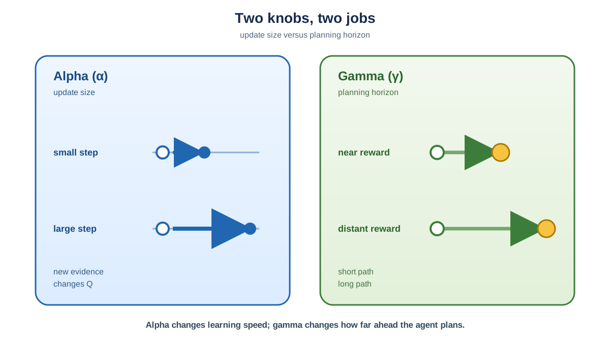
The learning rate, usually written as alpha (α), is the step size of each Q-value update. When your agent observes a new reward, alpha decides how much that observation moves the old estimate. A high alpha means the new observation heavily overwrites what the agent already believed. A low alpha means the agent nudges its belief only slightly.

The discount factor, usually written as gamma (γ), is the planning horizon. It decides how much future rewards count when the agent evaluates an action. A gamma near 1 means rewards far in the future matter almost as much as rewards now. A gamma near 0 means the agent mostly cares about what it can get immediately.

Here is the image I keep in my head: alpha is how fast you walk toward a target. Gamma is how far down the road you are willing to look before choosing a direction. You can walk quickly toward a short-sighted goal, or you can walk slowly toward a distant one. The two choices are independent.

The failure modes are different too. Alpha too high causes oscillation or divergence—the agent overreacts to single pieces of luck. Gamma too low makes the agent short-sighted—it settles for whatever reward is closest, even when a better path exists further ahead.

You already know the Q-update rule and how discounting works from earlier experiments. This article is about watching those two numbers change behavior in practice.

Setting Up One Baseline Before You Change Anything

Here is the discipline that makes this experiment worth running: change one variable at a time, and restore the baseline between changes.

Pick a small tabular environment you already know—a tiny grid or corridor task where you can watch the agent learn. You want something small enough that you can run many episodes quickly and inspect the final policy by hand.

Start with a baseline: a moderate alpha like 0.1 and a moderate gamma like 0.9. Keep exploration settings fixed. Run the experiment and record two things: the learning curve (average return per episode) and the final policy the agent settles on.

That baseline is your reference point. Every later run gets compared against it. If you change alpha and gamma at the same time, you will not know which knob caused the behavior you are seeing. That is not a tuning problem—it is an experimental design problem.

Note: This controlled-change discipline is the same ablation habit you use when comparing any two RL setups. Run the baseline first. Change one thing. Restore. Change the next thing.

Varying the Learning Rate While Gamma Stays Fixed

Keep gamma at 0.9. Now run the same experiment with a low alpha, like 0.01.

Watch the learning curve. It rises slowly. The agent needs many more episodes to converge than it did at baseline. But the curve is smooth—no wild swings between episodes. Each new observation barely moves the Q-values, so the agent's estimates drift gradually toward the truth.

Now run it with a high alpha, like 0.5 or 0.9.

The curve moves fast at first. The agent seems to learn quickly. But look closer: the curve overshoots, oscillates, and looks noisy before it settles. A single lucky or unlucky episode can swing the Q-values hard because each new reward heavily overwrites the old estimate.

Here is the mechanism: with a large alpha, the agent trusts each new observation almost completely. That is an advantage when the observation is informative and a disaster when it is misleading. One lucky episode can make the agent overvalue an action it has only tried once.

Watch for the symptom that matters: does the final policy converge to the same answer as the baseline, or does the instability prevent it from settling? Sometimes a high alpha still finds the right policy eventually. Sometimes it keeps thrashing and never quite lands.

The interpretation is not that high alpha is bad and low alpha is good. The learning rate trades speed against stability. A low alpha is slow but steady. A high alpha is fast but fragile. Your job is to find the value that converges quickly enough without oscillating.

Restoring the Baseline, Then Varying the Discount Factor

Put alpha back to 0.1. Now keep it fixed and change gamma instead.

Run the experiment with a low gamma, like 0.5.

The agent becomes short-sighted. It settles for immediate rewards even when a better long-term path exists. In a corridor task where the goal is at the far end, a low-gamma agent may learn to hover near a small intermediate reward instead of pushing through to the larger payoff. The learning curve may look fine—the agent is learning, and learning quickly. But the policy it settles on is wrong for the task.

Now run it with a high gamma, like 0.99.

The agent weighs distant rewards more heavily. It may take longer routes that pay off later. In that same corridor task, a high-gamma agent will learn to pass up the small immediate reward because it can see the larger one ahead. The policy looks different—not just learned faster or slower, but genuinely different in what it considers optimal.

Here is the mechanism: gamma changes which policy looks optimal, because it changes how the return is summed. With a low gamma, rewards ten steps away barely count. With a high gamma, they count almost as much as rewards now. The agent is not learning worse or better—it is optimizing a different objective.

Watch for the symptom that matters: the final policy itself differs, not just how fast it was reached. That is the signature of a discount-factor change. The learning rate changes the journey. The discount factor changes the destination.

Common mistake: Do not assume a very high gamma is always better. Distant rewards are harder to attribute reliably. The further the reward, the more steps of noise the agent must see through to connect an action to its consequence. A gamma near 1 can make value estimates harder to learn, even when the task rewards long-horizon planning.

Reading the Learning Curves Side by Side

Now lay out your runs: baseline, low alpha, high alpha, low gamma, high gamma. Read them as a set.

A healthy learning curve rises steadily and then flattens, with shrinking variance across episodes. Early episodes are noisy because the agent is exploring. As it learns, average return climbs and the spread between runs narrows.

Distinguish "learning faster" from "learning better." A steep curve can still settle on a worse policy. The high-alpha run may climb quickly and then oscillate around a mediocre result. The low-gamma run may climb smoothly toward a short-sighted policy. Speed of learning tells you nothing about the quality of the destination.

Do not judge from a single episode or a single seed. One lucky run can make a bad configuration look good. If you want reliable conclusions, run each configuration several times with different random seeds and compare the typical behavior, not the best episode.

Here is a decision rule for reading your curves:

• If the curve is slow but smooth, raise alpha a little.
• If the curve is noisy or oscillating, lower alpha.
• If the policy looks short-sighted, raise gamma.
• If the agent struggles to attribute distant rewards, lower gamma.

These two knobs answer different questions. Tune them for different symptoms.

What Each Knob Is Really Telling You

Here is the lesson compressed into one line: alpha changes how quickly the agent updates its beliefs; gamma changes which beliefs look worth holding.

When should you raise alpha? When the environment is stable, episodes are cheap, and you want faster convergence. The agent can afford to trust each observation because the world is not changing under it.

When should you lower alpha? When the curve oscillates, or when you suspect a single lucky episode is distorting the estimates. The agent needs to be skeptical of individual observations because they are noisy.

When should you raise gamma? When the task rewards long-horizon planning and the environment is learnable enough to support it. The agent needs to see the distant payoff to bother pursuing it.

When should you lower gamma? When episodes are long, rewards are sparse, or distant rewards are too hard to attribute reliably. The agent cannot learn from a reward it cannot connect to an action.

One boundary worth naming: in tabular RL, these effects are clean and observable. The Q-values live in a table, so you can watch exactly how each update moves them. In deep RL, the same knobs interact with function approximation, and the effects get messier. The intuition you build here carries forward, but the clean cause-and-effect you see in a small table does not survive contact with neural networks unchanged.

Your Next Experiment: Change One Thing and Watch

Turn this lesson into a habit. Run the same baseline again, and before each variation, write down what you predict. What will the learning curve look like with a low alpha? Will the high-gamma agent wait for the distant reward? Then run it and compare your prediction to the output.

The prediction step matters more than the run itself. It forces you to commit to a mental model before the evidence arrives. When your prediction is wrong, you learn something specific about where your model broke.

Here is a follow-up worth trying: set gamma near 1.0 on a task with a distant reward and watch whether the agent learns to wait for it. You will see the planning horizon stretch in real time as the agent stops grabbing nearby rewards and starts holding out for the better one ahead.

Keep a small log of which symptom led to which change. "Curve oscillated, lowered alpha." "Policy grabbed early reward, raised gamma." That log turns tuning from guesswork into evidence-based decisions, and it is the same controlled-change discipline you will carry into every deeper RL topic you tackle next.

References

Research updated Sep 9, 2026