State Abstraction in MDPs: Bisimulation and Safe State Merging

Merging states is not compression. It is a claim about the future, and most merges quietly change the problem.

Picture a tabular agent with a million states. The table is too big to fill, the backup loop is too slow to run, and somewhere in the middle of the state space you notice two states that "look the same." The instinct is immediate: merge them, shrink the table, move on. That instinct is where most silent bugs in value-based systems are born.

Here is the test this article builds toward. A merge is safe only if it preserves rewards and the distribution over future merged states, recursively, for every action. That single sentence is the whole idea. Everything below is the machinery that makes it checkable, plus one worked merge that survives and one plausible merge that does not.

I'll assume you already have the MDP tuple, discounted return, $V^\pi$ and $Q^\pi$, and the Bellman backup. If those are shaky, the formal map of MDPs and the derivation of the Bellman relationships are the two pieces to revisit first — this article leans on both without re-deriving them.

Why Merging States Is a Claim About the Future

The practical motivation is real. Tabular methods scale with the number of states: memory grows linearly, and the cost of a full sweep grows with $|S| \times |A|$. Aggregation is one of the few levers that attacks both at once. Fewer states means a smaller table, fewer samples to fill it, and cheaper planning.

But the lever has a hidden hinge. When you merge two states, you are asserting that no future decision can distinguish them. Not that they look alike — that they are behaviorally interchangeable. Feature similarity is a statement about the present. Interchangeability is a statement about every trajectory that could follow.

That distinction is the weak model to kill early. Two states can share every observable feature and still be different problems: one sits next to a cliff, the other next to a wall. Two states can look completely different and be the same problem: a corridor at sunrise and the same corridor at noon, when lighting is irrelevant to the task.

The stronger model is recursive. Two states are interchangeable only if, for every action, they yield the same immediate reward and lead to futures that are themselves interchangeable. Equivalence is defined in terms of equivalence. That self-reference sounds circular, but it is exactly what makes the condition checkable: it gives you a fixed-point equation, and fixed points can be computed.

Notation and the Abstraction Map

Fix the MDP $M = (S, A, P, R, \gamma)$ with finite $S$ and $A$, stationary dynamics $P(s' \mid s, a)$, expected reward $R(s, a)$, and discount $\gamma \in [0, 1)$. State values $V^\pi$ and action values $Q^\pi$ are the usual discounted expectations.

An abstraction is a surjective map $\phi: S \to Z$ onto a smaller set $Z$ of abstract states. Each $z \in Z$ is an equivalence class — a block — of ground states, and $\phi(s) = z$ means state $s$ belongs to block $z$.

The abstraction induces a new decision process on $Z$. The natural lift averages over the members of a block:

$P_\phi(z' \mid z, a) = \frac{1}{|z|} \sum_{s \in z} \sum_{s' \in z'} P(s' \mid s, a)$

$R_\phi(z, a) = \frac{1}{|z|} \sum_{s \in z} R(s, a)$

Warning: The induced process is not automatically Markov. If two states inside a block have different next-state distributions, the block's transition probabilities depend on which member you are actually in — information the abstract state has thrown away. The abstract process can be non-Markov even when the ground process is perfectly Markov.

This is where two ideas get conflated. State aggregation is a representation choice: you picked a map $\phi$. Bisimulation is a correctness condition on that choice. Aggregation is what you did; bisimulation is whether it was allowed.

Exact Conditions: Reward Preservation and Transition Preservation

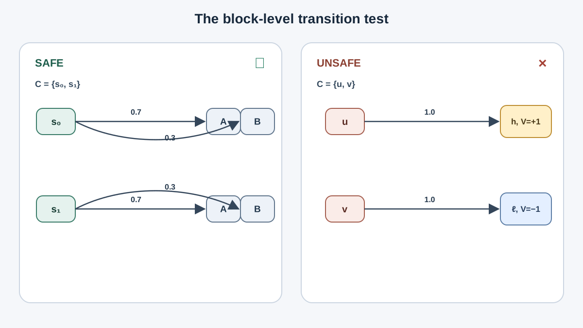
Two conditions define a bisimulation relation on the ground states. Both must hold for every action.

Reward preservation. For all $s, s' \in S$ with $\phi(s) = \phi(s')$, and every $a \in A$:

$R(s, a) = R(s', a)$

Same action, same immediate payoff. This forbids merging a state that pays $+1$ with one that pays $-1$ under the same action, no matter how similar their transitions look.

Transition preservation. For all $s, s'$ with $\phi(s) = \phi(s')$, every $a \in A$, and every abstract target $z \in Z$:

$\sum_{s'' \in z} P(s'' \mid s, a) = \sum_{s'' \in z} P(s'' \mid s', a)$

Read the left side carefully: it is the total probability mass that action $a$ in state $s$ sends into block $z$. The condition requires that mass to match for every block.

The block-level phrasing is not a technicality. It is the permission slip. The merge is allowed to reshuffle which member of a block you land in — that is invisible to the abstract agent. What it cannot do is change how much probability flows into each block. If $s$ sends 0.9 of its mass into block $z_1$ and $s'$ sends 0.4, the two states are not interchangeable, even if they both sometimes reach $z_1$.

Recursive closure. The conditions above are stated over blocks, and blocks are made of states that must themselves satisfy the conditions. That closure is what makes this bisimulation rather than one-step aggregation. A one-step check can pass while the recursion fails two steps later, because the blocks you land in are not internally consistent.

What each condition rules out is clean. Reward mismatch breaks the immediate comparison — the agent cannot even rank actions within the block. Transition mismatch breaks the value of the future even when rewards agree perfectly, because the two states face different distributions over where they end up.

Worked Example: A Valid Merge

Take a four-state corridor. States $s_0, s_1, s_2, s_3$ in a line, two actions: left and right. Moving right from $s_3$ or left from $s_0$ stays put. Reward is $+1$ on entering $s_3$ and $0$ otherwise. Discount $\gamma = 0.9$.

Now consider merging $s_0$ and $s_1$ into a single block $z_{01} = \{s_0, s_1\}$, keeping $s_2$ and $s_3$ as singleton blocks.

Reward check. $R(s_0, \text{left}) = R(s_1, \text{left}) = 0$ and $R(s_0, \text{right}) = R(s_1, \text{right}) = 0$. Rewards match for both actions.

Transition check. Compute block-level mass for each action.

From	Action	Mass into $z_{01}$	Mass into $s_2$	Mass into $s_3$
$s_0$	right	0	1.0	0
$s_1$	right	0	1.0	0
$s_0$	left	1.0	0	0
$s_1$	left	1.0	0	0

Both rows match for both actions. The merge is valid.

Now solve. On the ground MDP, $V(s_3) = 0$ (absorbing, no further reward), $V(s_2) = 0.9 \cdot 1 = 0.9$, $V(s_1) = 0.9 \cdot 0.9 = 0.81$, $V(s_0) = 0.9 \cdot 0.81 = 0.729$.

On the abstract MDP with block $z_{01}$, the block's value under the optimal policy is the same $0.729$ for both members, because both members have identical reward and identical block-level transitions. The optimal action in the block is right for both. The abstraction bought a smaller table without buying a different problem.

That is what planning equivalence looks like in numbers: same values, same policy, fewer rows.

Counterexample: A Merge That Looks Fine and Is Not

Now the trap. Two states, $u$ and $v$, with identical rewards for every action — say $R(u, a) = R(v, a) = 0$ for all $a$. They look mergeable. They are not.

Let the dynamics differ. From $u$, action $a$ sends you to a high-value state $h$ with probability 1. From $v$, action $a$ sends you to a low-value state $\ell$ with probability 1. Rewards are identical; futures are not.

Solve the ground MDP with $\gamma = 0.9$, $V(h) = 10$, $V(\ell) = 0$:

$V(u) = 0 + 0.9 \cdot 10 = 9, \qquad V(v) = 0 + 0.9 \cdot 0 = 0$

The merged block averages the transition: half the mass to $h$, half to $\ell$. The abstract value becomes:

$V_\phi(z_{uv}) = 0 + 0.9 \cdot (0.5 \cdot 10 + 0.5 \cdot 0) = 4.5$

The merged value is wrong for both states. It overstates $v$ by 4.5 and understates $u$ by 4.5. Any policy computed on the abstract MDP is optimizing a problem that does not exist.

Second variant: transitions match, rewards do not. Let $u$ and $v$ have identical next-state distributions for every action, but $R(u, a) = +1$ and $R(v, a) = -1$. The merged reward is $0$. The abstract MDP now prefers an action that is optimal in the average and suboptimal in the ground problem — the agent learns a policy that is worse than either state deserved.

Common mistake: Treating a failed merge as a compression error. It is not. It is a change of objective. The abstract MDP is a different problem, and its optimal policy is optimal for that different problem.

What the Equivalence Guarantees — and What It Does Not

Under the two conditions, with the recursion closed, optimal values and an optimal policy transfer between the ground MDP and the abstract MDP. That is the payoff: you can plan on the small problem and act on the large one.

The result rests on assumptions worth naming. Finite state and action sets. Stationary dynamics and rewards. A fixed discount. Exact knowledge of $P$ and $R$. Drop any of these and the guarantee weakens.

Estimated or drifting models are the common failure. If your $P$ and $R$ come from samples, the equality checks become approximate, and small estimation errors can flip a merge from valid to invalid. Non-stationary rewards break the fixed-point structure entirely. Continuous or high-dimensional state spaces make exact partitions brittle: the relation is hypersensitive to infinitesimal changes in rewards or dynamics, so a partition that holds today may not hold after one more update.

The relaxation path is the bisimulation metric. Instead of asking whether two states are exactly equivalent, you ask how far apart they are. The metric replaces the binary partition with a distance that varies smoothly as rewards and dynamics change, and a distance of zero recovers the exact merge. That smoothness is what makes the idea usable when the MDP is estimated or continuous — you trade exactness for robustness.

The honest boundary: exact bisimulation is a correctness criterion for a known finite MDP. It is not a general recipe for learning good representations from raw observations.

When to Reach for This — and When Not To

Use it when you have a known or well-estimated finite MDP, a state space too large to tabulate, and a need to prove that aggregation is safe. Use it as a diagnostic when a learned representation underperforms: check whether the encoder is collapsing states that are not behaviorally equivalent, because that is a silent objective change, not a capacity problem.

Do not reach for it first on a raw pixel environment. Exact partitions are impractical there, and the metric relaxation is the realistic tool. Do not treat it as a substitute for a good state representation — it is a test you run on a representation you already have.

The practical check is mechanical. Before merging any pair of states, write down two equalities for every action: reward equality, and block-level transition equality into every abstract target. If either fails, you have not simplified the problem. You have replaced it.

That is the decision rule. Write the equalities. Check them. A failed check is evidence, not an inconvenience.

When the MDP is estimated rather than known, the next step is replacing the exact partition with a bisimulation distance — the same recursive idea, softened into a metric that tolerates small perturbations. Take a small MDP you already understand, propose a merge, and verify or falsify it numerically. The exercise is short, and it will change how you look at every state table you build afterward.