
Optimism and Confidence Bonuses in Tabular Reinforcement Learning
An agent that has seen an action once does not know its value. It knows one sample. Optimism is the discipline of treating thin evidence as a reason to…

Key topics
An agent that has seen an action once does not know its value. It knows one sample. Optimism is the discipline of treating thin evidence as a reason to look again — and confidence bonuses are how that discipline becomes arithmetic.
What "Optimistic" Actually Commits You To
Picture two agents stuck in the same corridor. The first keeps re-taking a mediocre action because its estimate is confidently wrong: it saw a decent reward once, stopped looking, and never learned the action was a trap. The second refuses to touch an action it has seen only once, because a single low sample convinced it the action is bad. Both fail for the same reason — they treat thin evidence as settled fact.
The principle of optimism in the face of uncertainty (OFU) is the formal answer. It says: act as if the environment is the most favorable one still consistent with the data you have observed. You do not add a big number to unseen things and hope. You ask which value function the data has not yet ruled out, and you act on the best one still standing.
That framing names both failure directions. Under-optimism means the agent never explores, gets stuck on a known-mediocre action, and pays for it forever. Over-optimism means the agent chases noise — inflating every uncertain estimate so hard that it wanders off after statistical ghosts. The goal is to over-estimate the true value without becoming inaccurate. Optimism is a claim about what the data permits, not a mood.
You already know the exploration-exploitation tradeoff and you have seen bonuses built from counts, novelty, and prediction error. This article asks a narrower question: how does an uncertainty term become a concrete value estimate, and when does that construction stop being trustworthy?
Everything below assumes a finite, tabular setting: finitely many states and actions, with a visit count available for every state-action pair. That assumption is load-bearing. Remove it and the guarantees change character, which is exactly what the last section is about.
Knowledge check
Check your understanding
Answer this question before you continue.
Notation and the Confidence Interval
Let the environment be a Markov decision process : states , actions , transition function , reward function , discount . For a state-action pair , let be the number of times we have taken action in state , and let
be the empirical mean of the immediate rewards observed there.
Here is the scope decision that matters, and it is where most beginner explanations quietly cheat. In a general MDP, the action value is not the mean of immediate rewards. It is the expected discounted sum of everything that follows:
So is not an estimate of . It is an estimate of one term inside it. To keep the derivation honest, I will work the one-step case first — a bandit-like setting where the action's value really is its immediate reward mean — and then show what full tabular RL adds. That separation is the difference between a formula you can trust and a formula you have memorized.
The one-step case. Suppose rewards for a fixed pair are drawn from a distribution with mean and bounded range. The sample mean is unbiased for but noisy. Hoeffding's inequality gives, with probability at least ,
Read that as a statement about width. The true mean lies inside an interval centered on our estimate, and the half-width shrinks as . Fewer visits, wider interval. More visits, narrower interval. That half-width is the bonus:
Each factor has a job. The constant sets the overall scale. The term pays for confidence: if you want the interval to hold simultaneously across many state-action pairs, the bound must loosen logarithmically with the number of claims you are making. And controls the width directly — this is the term that makes the bonus self-extinguishing.
The assumptions are plain: rewards are bounded, and samples for a given pair come from a fixed distribution. Unbounded rewards break the concentration argument. A drifting distribution makes old samples stale evidence, and the interval becomes a lie.
What full tabular RL adds. In an MDP, uncertainty lives in two places: the reward mean and the transition probabilities. A state-action pair you have visited once gives you a shaky estimate of where you land next, and that shakiness propagates through the Bellman recursion into the value estimate. The standard tabular construction — the one behind algorithms like UCBVI — adds a bonus at the value level, roughly
where carries the combined reward-and-transition uncertainty and is the optimistic value of the next state. The bonus is no longer a single interval around a mean; it is a term inside a recursion that must be solved by dynamic programming. The intuition survives — wide uncertainty, high bonus — but the arithmetic does not collapse to one square root.
Contrast this with the bonus families you have already met. A count-based or novelty bonus rewards being unseen — it pays for visiting anything new. A confidence bonus rewards being uncertain in a way that shrinks with evidence. Novelty never runs out; a confidence interval closes.
Knowledge check
Check your understanding
Answer this question before you continue.
A Worked Example in the One-Step Case
Let us make the arithmetic concrete, staying inside the one-step scope where the derivation is exact. Consider a single decision point with two actions, and . Action pays a steady reward of every time. Action pays a reward drawn from a fixed distribution with mean — sometimes , sometimes , occasionally more. The agent does not know either mean.
Take and for simplicity, so the bonus is . Suppose the agent has taken twenty-five times and exactly once, and that single sample happened to come back as .
| Action | Empirical mean | Bonus | Optimistic | |
|---|---|---|---|---|
| 25 | 1.00 | 0.20 | 1.20 | |
| 1 | 0.00 | 1.00 | 1.00 |
The greedy-over-optimistic-values rule picks the largest . Here wins, to . The agent keeps taking the reliable action. That is correct given the evidence: one bad sample is weak evidence, but it is not no evidence, and the wide interval around still falls short.
Now push the counts. Suppose the agent has taken four times, and the samples average — which, in this construction, is exactly the true mean.
| Action | Empirical mean | Bonus | Optimistic | |
|---|---|---|---|---|
| 25 | 1.00 | 0.20 | 1.20 | |
| 4 | 0.25 | 0.50 | 0.75 |
The bonus on has shrunk from to , and its optimistic value is now clearly below . The empirical mean has taken over. This is the mechanism you should be able to narrate: an under-visited action wins the argmax when its interval is wide enough to cover the gap, and loses once enough visits narrow the interval below that gap.
One more step shows the flip. Suppose has been visited only twice, with samples averaging :
| Action | Empirical mean | Bonus | Optimistic | |
|---|---|---|---|---|
| 25 | 1.00 | 0.20 | 1.20 | |
| 2 | 0.25 | 0.71 | 0.96 |
Still . But drop 's count to five and the picture changes:
| Action | Empirical mean | Bonus | Optimistic | |
|---|---|---|---|---|
| 5 | 1.00 | 0.45 | 1.45 | |
| 2 | 0.25 | 0.71 | 0.96 |
The gap between the two empirical means is . The bonus gap is . The bonus does not close a gap that large. This is the honest lesson: optimism is not magic. It resolves ties and near-ties in favor of the less-visited action. It does not override a decisive difference in observed reward.
Knowledge check
Check your understanding
Answer this question before you continue.
Why the Bonus Shrinks, and What That Buys You
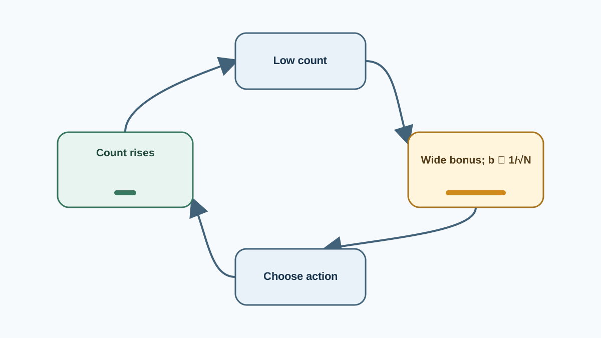
The decay is the whole point. Exploration is front-loaded and self-extinguishing. The agent does not need a separate epsilon schedule to stop exploring — the bonus shrinks on its own as evidence accumulates. Every visit to a pair makes that pair less interesting to an optimistic agent.
This connects to the regret framing without requiring a proof. An optimistic agent's cumulative shortfall against the optimal policy is bounded because the agent can only stay wrong about a pair for as long as the interval is wide. Once the interval closes, the estimate is accurate enough that acting greedily is nearly optimal. The agent's mistakes are self-limiting.
Compare that to epsilon-greedy, which explores at a constant rate forever. An epsilon-greedy agent keeps paying a tax on actions it already understands, because its exploration does not depend on what it knows. A confidence bonus spends its exploration budget where the interval is still wide — which is why it is sample-efficient in the tabular regime.
Where the Assumptions Break
The construction above is clean because the setting is clean. Here is where it stops meaning what it claims.
Function approximation. Once is a neural network, does not exist. You can build pseudocounts or ensembles as proxies, but the interval they produce is not the interval the theory assumes. The concentration argument was about a sample mean over independent draws from a fixed distribution; a network's uncertainty estimate is a different object wearing the same name.
Averaging standard deviations instead of variances. This is a specific, well-documented flaw. When you propagate uncertainty across possible next states, you should average variances, not standard deviations. Averaging standard deviations produces an incoherent uncertainty estimate: for any fixed bonus scale , there are visit counts for which the agent explores when it is not actually uncertain, and fails to explore when it is. The bonus no longer tracks data sufficiency.
Non-stationary data. If the reward distribution shifts, old counts are stale evidence. The interval computed from them is too narrow, and the agent becomes confidently wrong — the exact failure we opened with, now dressed in a formula.
Reward and bonus scale interaction. A bonus tuned for one reward magnitude silently becomes either negligible or dominant when the reward scale changes. Nothing errors out; the agent just explores too little or too much.
Practical rule: treat the bonus as a claim about data sufficiency. Before trusting it, check whether your uncertainty estimate actually shrinks when you collect more data in your setting. If it does not, the bonus is decoration.
Knowledge check
Check your understanding
Answer this question before you continue.
Optimism or Randomization?
There is a second family of exploration methods worth placing beside optimism. Optimism picks the best value consistent with the data and acts greedily on it. Randomization samples a plausible value function from a posterior and acts greedily on the sample. Both are principled; they differ in what they do with uncertainty.
The honest empirical picture: on some tabular problems, randomized exploration learns faster than optimistic exploration. In comparisons on problems like RiverSwim, posterior-sampling methods have been observed to learn considerably faster than optimistic ones. Optimism is not automatically the stronger choice.
There is also evidence that the most effective degree of optimism varies both across tasks and over the course of learning. That argues against a single fixed bonus scale and in favor of treating optimism as a dial rather than a constant.
A decision rule: use optimism when you can build a defensible uncertainty estimate and you want deterministic, reproducible behavior. Consider randomization when your uncertainty model is itself a guess — sampling from a rough posterior is more forgiving than committing to a wrong interval.
What to Do Next
Before you add a confidence bonus to anything, write down what your uncertainty estimate is actually measuring. Is it a count of independent samples from a fixed distribution? Or is it a proxy that happens to correlate with novelty? The answer determines whether the bonus means what the theory says it means.
Then instrument it. Run a small tabular experiment and log , the bonus, and the value estimate side by side. Watch whether exploration decays for the reason the theory predicts — because the interval closed — or for some other reason, like the bonus being swamped by the reward scale or the counts going stale. The gap between those two explanations is where most real exploration bugs live.
If you want to see this in motion before adding any bonus, start with a plain tabular agent and watch its Q-values settle. The confidence bonus only makes sense once you can see what it is perturbing.
Knowledge check
Final check
Finish the article by checking the ideas you just learned.
References
Build a stronger RL mental model
Use structured resources to connect equations, algorithms, and observable agent behavior.


