
Prioritized Experience Replay: Deriving Sampling Probabilities and Importance Weights
You add prioritized replay. Training speeds up. Loss drops faster than it ever did with uniform sampling. Then, a few hundred thousand steps later, the…

Key topics
You add prioritized replay. Training speeds up. Loss drops faster than it ever did with uniform sampling. Then, a few hundred thousand steps later, the value estimates settle somewhere slightly wrong — not catastrophically wrong, just wrong enough that the policy is worse than the uniform-replay baseline you were trying to beat.
Nothing crashed. Nothing diverged. The sampler quietly changed the distribution you were averaging over, and nobody paid the invoice.
That invoice has two line items: the sampling probability and the importance weight. This article derives both. By the end, you should be able to compute them by hand for a small buffer and explain why the correction exists at all.
What Prioritized Replay Actually Changes
Uniform replay samples each stored transition with probability , where is the current number of transitions in the buffer. The Q-learning update is then an average over that distribution. That average is the thing you are implicitly trusting.
Prioritized replay replaces that distribution with one proportional to a priority score. In the common variant, the priority is the absolute temporal-difference (TD) error:
A large TD error means the current value estimate is wrong at that transition. The intuition — "sample the surprising stuff more" — is correct as far as it goes. But it is not the whole story, and treating it as the whole story is exactly how you end up with the drift described above.
The assumption we will hold fixed for the derivation: the buffer is fixed, the policy is fixed, and we are asking what the expected update converges to under a non-uniform sampler. That is the cleanest setting to see the bias. Real training violates all three, but the bias does not disappear when they move — it just gets harder to isolate.
Two knobs control everything. Alpha () controls how much prioritization you apply. Beta () controls how much correction you apply. We will derive both.
Notation and the Two Distributions
Before any formula, name the objects.
| Symbol | Meaning |
|---|---|
| Current number of transitions in the buffer (not capacity) | |
| Index of a stored transition | |
| Priority of transition | |
| Priority exponent, | |
| Probability of sampling transition | |
| Importance-sampling exponent, | |
| Importance weight for transition | |
| Small constant added to priorities so nothing is unsampleable |
The central tension is this: there is a distribution you sample from, and a distribution you want to average over. Prioritized replay makes those two different. The importance weight is what reconciles them.
The sampling rule is:
Read it aloud: raise each priority to a power, then normalize so the probabilities sum to one. That is the whole formula.
Two boundary cases matter. At , every , so — uniform sampling. At , sampling is fully proportional to priority. Everything between is a dial.
The term is not cosmetic. Without it, a transition whose TD error is exactly zero gets and can never be sampled again. It becomes a permanent resident of the buffer that contributes nothing. Small keeps every transition reachable.
The target distribution is the uniform distribution over the buffer. That is what the unweighted update implicitly assumes, and it is what we are trying to recover.
Deriving the Sampling Probability
Start from intent, not from the formula. We want a monotone, controllable mapping from priority to sampling chance. Monotone means higher priority never gets sampled less. Controllable means one knob that slides between "ignore priorities" and "trust them completely."
A power law satisfies both. A linear map would give you proportional sampling but no dial — you would have to redesign the formula to get uniform behavior back. The power law degrades gracefully: set and you are exactly uniform, no special case required.
Normalization is forced by probability. The probabilities must sum to one, so:
Now work a small buffer by hand. Five transitions with priorities $1, 4, 9, 16, 25\alpha = 0.6$.
| 1 | 1 | 1.000 | 0.056 |
| 2 | 4 | 2.297 | 0.129 |
| 3 | 9 | 3.737 | 0.210 |
| 4 | 16 | 5.278 | 0.296 |
| 5 | 25 | 6.899 | 0.387 |
| 19.211 | 1.000 |
The highest-priority transition is sampled roughly seven times as often as the lowest. Now move the dial.
At , every . Uniform. At , the probabilities become $0.018, 0.073, 0.164, 0.291, 0.455$ — the top transition is sampled twenty-five times as often as the bottom. The dial is not subtle.
One implementation note: naive sampling from costs per draw because you must scan the cumulative distribution. Production implementations use a sum-tree to get sampling and updates, often combined with stratified sampling to reduce variance. That is an engineering detail, not a mathematical one, but it is why you rarely see the raw formula in code.
Knowledge check
Check your understanding
Answer this question before you continue.
Why Non-Uniform Sampling Biases the Update
Here is the mechanism, stated plainly. The update is an expectation over sampled transitions. Changing the sampler changes the expectation — not just the variance.
High-priority transitions get counted many times per epoch. Their gradient contribution is inflated relative to their true share of the buffer. If you train long enough with a fixed policy and a fixed state distribution, the value estimate converges toward the solution of a reweighted objective, not the original one.
This is the part that catches people. Prioritization is often described as a variance-reduction trick, in the same family as importance sampling in Monte Carlo estimation. It is not. It is a deliberate change to the distribution you average over, and that change has a real cost.
The failure mode is specific: uncorrected prioritization looks faster early, because the samples with the largest learning signal dominate the gradient. Then it settles at the wrong place, because the objective it is actually optimizing is not the one you wrote down. The drift is not mysterious. It is the sampler's distribution showing up in the fixed point.
Knowledge check
Check your understanding
Answer this question before you continue.
Deriving the Importance Weight
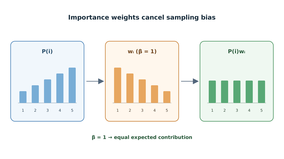
Importance sampling in one line: to estimate an expectation under distribution using samples drawn from distribution , weight each sample by .
Here, is uniform — — and is . So the raw weight is:
Introduce as a partial correction:
At , the correction is full and the estimator is unbiased with respect to the uniform distribution. At , every weight is 1 and you are back to the uncorrected case. Everything between trades a little bias for a little stability.
Then normalize within the mini-batch:
Dividing by the maximum weight keeps the largest weight at 1 and prevents gradient magnitudes from exploding when a rare transition receives a very large raw weight. This is a stability measure, not a mathematical necessity — the expectation is unchanged, but the variance of the gradient is much better behaved.
The annealing schedule is the practical part. typically starts below 1 and rises toward 1 over training. Early updates benefit from aggressive prioritization because the value estimates are far from correct and the largest TD errors carry the most useful signal. Late updates need unbiased targets because the estimates are close and the remaining bias is what determines the final fixed point.
Common mistake: Treating as a fixed hyperparameter. If stays at 0.4 for the entire run, you never fully pay back the sampling debt, and the drift described at the top of this article is exactly what you get.
Knowledge check
Check your understanding
Answer this question before you continue.
Worked Example: Weights for a Five-Transition Buffer
Reuse the five priorities from earlier. The values at are $0.056, 0.129, 0.210, 0.296, 0.387(N \cdot P(i))^{-\beta}\beta = 0.4\beta = 1.0$, then apply max-normalization.
| at | normalized | at | normalized | ||
|---|---|---|---|---|---|
| 1 | 0.056 | 1.716 | 1.000 | 3.571 | 1.000 |
| 2 | 0.129 | 1.214 | 0.708 | 1.550 | 0.434 |
| 3 | 0.210 | 1.000 | 0.583 | 0.952 | 0.267 |
| 4 | 0.296 | 0.869 | 0.506 | 0.676 | 0.189 |
| 5 | 0.387 | 0.788 | 0.459 | 0.517 | 0.145 |
Read the result. The highest-priority transition gets weight 1.0 in both cases — it is the reference point after normalization. The lowest-priority transition is down-weighted to 0.459 at and to 0.145 at . The correction is doing exactly what the bias argument demanded: pulling the inflated contribution of high-priority samples back toward their true share.
At , every weight would be 1. That is the uncorrected case, and it is the one that drifts.
Sanity check: if all five priorities were equal, every would be , every raw weight would be , and every normalized weight would be 1 regardless of . When the sampling distribution is already uniform, there is nothing to correct.
Knowledge check
Check your understanding
Answer this question before you continue.
Where the Derivation Breaks Down
The formulas rest on assumptions that real training violates. Knowing which ones matters more than knowing the formulas.
Stale priorities. A transition's TD error is recorded when it is sampled. A transition that becomes relevant later — because the policy changed, or because the agent reached a new region of state space — can stay buried under an old low priority. Periodic priority refresh and a small mitigate this, but they do not eliminate it.
Sampling with replacement. Most reference implementations sample with replacement, which means the same high-priority transition can land in a mini-batch several times. Its influence is then inflated beyond what the importance weight corrects, because the weight was derived for a single draw. Sampling without replacement is an option, but it changes the distribution in ways the standard derivation does not cover.
The weight corrects the sampler, not the target. The importance weight fixes the distribution mismatch introduced by prioritization. It does nothing about the fact that the TD target is a bootstrapped estimate. That instability is a separate problem with separate tools.
Recurrent agents. If your value function carries hidden state, random access to a transition requires reconstructing the correct hidden state by replaying the episode up to that point. Some frameworks simply do not support prioritized replay for recurrent agents, and the ones that do pay a real cost per sample.
Hyperparameter sensitivity. Performance depends noticeably on , , and . These are tuning parameters with consequences, not defaults to ignore.
Choosing Alpha and Beta in Practice
The derivation gives you the dials. Here is how I would turn them.
Start with and annealed from roughly to . These are common starting points, not laws.
If training is unstable or value estimates drift, raise toward 1 before touching . The drift is almost always unpaid sampling debt, and is the payment.
If learning is slow and the buffer is large with many near-duplicate transitions, is the dial to raise. More prioritization means more focus on the transitions that still have something to teach.
When not to use it: small buffers, short runs, or settings where uniform replay already converges. The extra machinery buys nothing there and adds two hyperparameters plus a sum-tree to maintain.
Debugging rule: Log the distribution of importance weights. If most weights are near zero and a few are near one, the correction is doing heavy lifting — which usually means the priorities are too aggressive for the current . If every weight is near one, the priorities are nearly uniform and prioritization is not doing much at all.
The opening symptom — faster early, wrong later — was never mysterious. Prioritization changes the distribution you average over. The importance weight is the receipt. If you never pay it, the fixed point moves.
The next concrete move: instrument your own replay buffer. Log the priorities and the importance weights for a few thousand sampled batches. Plot both distributions. If the weight distribution does not look like the inverse of the priority distribution you intended, the correction is not doing what you think it is — and you now have the derivation to explain why.
Knowledge check
Final check
Finish the article by checking the ideas you just learned.
References
Build a stronger RL mental model
Use structured resources to connect equations, algorithms, and observable agent behavior.


