
Build a Small DQN Agent in Python: Replay Buffers and Target Networks
You can explain replay buffers and target networks. You have never watched a loss curve flatline while episode return refuses to move. That gap between…

Key topics
You can explain replay buffers and target networks. You have never watched a loss curve flatline while episode return refuses to move. That gap between explaining DQN and running one is where the real learning starts.
This tutorial builds the smallest honest DQN: a small environment, a small MLP, a ring-buffer replay, and a lagged target network. Then we break it on purpose so the failure signals stop being abstract.
The conceptual bridge is short. Bootstrapping plus function approximation creates a moving target: you train the network toward a target that the network itself produces. Replay decorrelates the data; a lagged target network freezes the target long enough for the online network to chase something stable. That is the whole mechanism. Everything below is wiring it up and reading what comes out.
What You Are Actually Building
Target a small discrete-action task where the state is a short vector and there are two or three actions. CartPole-style environments fit exactly. The state is four numbers; the actions are left or right.
Dependencies: Python, PyTorch, Gymnasium (or an equivalent environment API), and NumPy. CPU is sufficient. At this scale a GPU adds setup friction and buys nothing.
Five moving parts:
- Q-network — maps a state vector to one Q-value per action.
- Target network — a lagged copy of the Q-network.
- Replay buffer — fixed-capacity store of past transitions.
- Epsilon-greedy selection — explore early, exploit later.
- Optimizer and loss — mean squared error against the Bellman target.
Success criterion, stated before any code: episodic return rises and stabilizes above a threshold within a few hundred episodes, and the loss does not diverge. If return stays flat and loss stays noisy, you have a diagnosable failure, not a mystery.
The Q-Network and the Target Network
The Q-network is a small MLP. Output shape matters more than depth: one value per action.
import torch
import torch.nn as nn

class QNetwork(nn.Module):
    def __init__(self, state_dim, action_dim, hidden=64):
        super().__init__()
        self.net = nn.Sequential(
            nn.Linear(state_dim, hidden),
            nn.ReLU(),
            nn.Linear(hidden, hidden),
            nn.ReLU(),
            nn.Linear(hidden, action_dim),
        )

    def forward(self, x):
        return self.net(x)
The target network is initialized as an exact copy, with gradients disabled on the target path:
online = QNetwork(state_dim, action_dim)
target = QNetwork(state_dim, action_dim)
target.load_state_dict(online.state_dict())
for p in target.parameters():
    p.requires_grad = False
Two update styles:
| Style | Mechanism | Tradeoff |
|---|---|---|
| Hard update | Copy online weights into target every N steps | Simple, but the target jumps discontinuously |
| Soft update (Polyak) | Blend target toward online each step | Smoother target, one more hyperparameter |
The target must not be updated by the same gradient step that trains the online net. That lag is the entire point. If the target moves with every gradient step, you are back to chasing a target that runs at your own speed.
Common mistake: Forgetting to detach the target computation. If you compute the Bellman target without
torch.no_grad()or without frozen target parameters, gradients flow into the target network and the lag silently disappears.
Knowledge check
Check your understanding
Answer this question before you continue.
The Replay Buffer: Store, Sample, Forget
Store transitions as (state, action, reward, next_state, done). The done flag is what stops bootstrapping across episode boundaries — without it, the agent learns that terminal states lead to more reward.
import random
from collections import deque

class ReplayBuffer:
    def __init__(self, capacity):
        self.buffer = deque(maxlen=capacity)

    def push(self, state, action, reward, next_state, done):
        self.buffer.append((state, action, reward, next_state, done))

    def sample(self, batch_size):
        batch = random.sample(self.buffer, batch_size)
        states, actions, rewards, next_states, dones = zip(*batch)
        return (
            torch.tensor(states, dtype=torch.float32),
            torch.tensor(actions, dtype=torch.int64),
            torch.tensor(rewards, dtype=torch.float32),
            torch.tensor(next_states, dtype=torch.float32),
            torch.tensor(dones, dtype=torch.float32),
        )

    def __len__(self):
        return len(self.buffer)
Capacity is a real hyperparameter, not a formality. Too small and the agent overfits to recent experience. Too large and old, stale transitions dilute the signal.
Uniform random sampling breaks the temporal correlation that destabilizes plain online Q-learning. Consecutive transitions are nearly identical; training on them in order is training on a batch of near-duplicates.
Warm-up matters. Do not start gradient updates until the buffer holds enough transitions. Early batches drawn from a nearly empty buffer are near-duplicates, and the loss you see is not informative.
Tip: Before trusting any loss number, print
len(buffer)and the shape of one sampled batch. Confirm sampling works before you debug anything else.
Knowledge check
Check your understanding
Answer this question before you continue.
The Training Loop and the Bellman Target
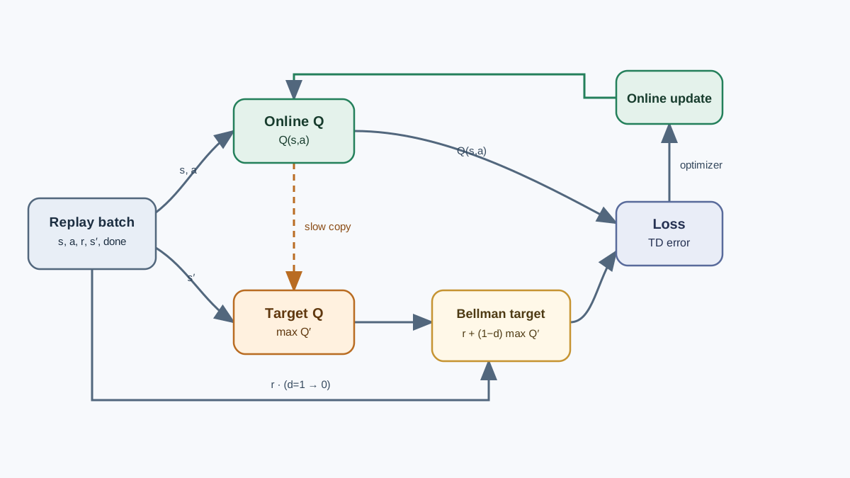
Per step: select an action with epsilon-greedy, step the environment, push the transition, sample a batch, compute the loss, step the optimizer.
The target computation is where most silent bugs live:
with torch.no_grad():
    next_q = target(next_states).max(dim=1).values
    targets = rewards + gamma * next_q * (1.0 - dones)

predicted = online(states).gather(1, actions.unsqueeze(1)).squeeze(1)
loss = nn.functional.mse_loss(predicted, targets)
Two details that break quietly if you get them wrong:
gathermust select the Q-value for the action actually taken, not the max. If you usemaxon the online network here, you are training the wrong quantity.(1.0 - dones)zeroes the bootstrap term at terminal states. Skip it and the agent learns that episodes never end.
Epsilon decay: explore broadly early, exploit later. The decay horizon is a real tuning knob. Decay too fast and the agent commits to a bad policy; decay too slow and it never exploits what it learned.
Log episodic return per episode, plus a rolling average and the loss. Trends are visible; single numbers are noise.
Knowledge check
Check your understanding
Answer this question before you continue.
Reading the Training Signals
The return curve shape tells you more than any single value. Flat-then-rising is normal. A permanently flat curve is the interesting case.
Loss is not a progress metric in RL. A falling loss with flat return is a classic and confusing pattern. The network is getting better at predicting targets that are themselves moving. Low loss means the network agrees with its own lagged copy, not that the policy improved.
Q-value magnitude drift is a warning. Exploding or collapsing Q estimates point at target or discount problems. If mean Q grows without bound, check whether the target is actually lagged.
Action distribution matters. If the agent picks one action almost always, exploration has collapsed or the network has saturated.
Log at minimum: episodic return, rolling average, mean Q, epsilon, and buffer size. Five numbers, one line per episode.
Knowledge check
Check your understanding
Answer this question before you continue.
Breaking It on Purpose: A Diagnosable Failure
Set the target update interval to every step — or point the target at the online network directly — and rerun.
Expected symptom: return oscillates or collapses while loss stays noisy or grows. The agent is chasing a target that moves with it.
Diagnosis path, in order:
- Is the target actually lagged? Print the target update counter. Confirm it fires on schedule.
- Are done flags handled? Check that terminal transitions zero the bootstrap term.
- Is the buffer being sampled at all? Print batch shapes and buffer length.
Second failure to try: shrink the buffer to a few hundred transitions. Watch the agent overfit to recent experience — return spikes then collapses as the buffer cycles through the same narrow slice of states.
Fix and confirm: restore the lagged target or the larger buffer, rerun, and compare curves side by side. The difference is the lesson.
One Modification Worth Trying Next
Double DQN is the natural next step. Use the online network to select the greedy action and the target network to evaluate it:
with torch.no_grad():
    best_actions = online(next_states).argmax(dim=1, keepdim=True)
    next_q = target(next_states).gather(1, best_actions).squeeze(1)
    targets = rewards + gamma * next_q * (1.0 - dones)
This reduces overestimation: vanilla DQN's max operator systematically picks the highest noisy estimate. Double DQN decouples selection from evaluation.
It fits here because it reuses the two networks you already built. The change is a few lines, not a rewrite.
Compare return curve and mean Q magnitude against the vanilla run, not just final score. A lower mean Q with the same return is the expected signature.
Where to stop: prioritized replay, dueling heads, and distributional variants are separate topics with their own failure modes. Do not stack them onto a working agent until you can explain what each one fixes.
What to Do Next
You now have a working agent, a short list of signals to log, and a rule for the next time training stalls: check the target lag, check the done flags, check the buffer before touching the learning rate.
The habit matters more than the hyperparameters. When return flatlines, the failure is almost never the learning rate. It is a broken assumption about what the target is, what the buffer holds, or what the done flag means.
Run the Double DQN modification. Compare the curves. Then pick one failure mode from this article, reproduce it deliberately, and watch the signal that tells you it broke. That is how the mechanism stops being theory and becomes something you can see.
Knowledge check
Final check
Finish the article by checking the ideas you just learned.
References
Build a stronger RL mental model
Use structured resources to connect equations, algorithms, and observable agent behavior.


