
Bellman Error With Function Approximation: Why Low Training Loss Can Mislead
Your value network's loss curve flattens to something that looks like zero. The run looks healthy. Then you watch the greedy policy walk straight into a…

Key topics
Your value network's loss curve flattens to something that looks like zero. The run looks healthy. Then you watch the greedy policy walk straight into a wall it has visited a hundred times.
The relief is understandable, and it is also the trap. A low training loss tells you the optimizer is fitting targets on the states it saw. It does not tell you the value function is correct. Those are different claims, and the gap between them is where most quiet value-function bugs live.
By the end of this article you will be able to read any Bellman-error number and say which of three errors it does and does not contain: approximation error, optimization error, and sampling error. Only the first is a property of the function class itself. The other two are properties of your training run.
The Loss Curve Is Not a Value Report
Here is the weak model I want to replace: low loss means the values are right.
A loss is a fit to targets on a data distribution. Value accuracy is a property of the function over the entire state space. Those two things coincide only under conditions most practitioners never check.
Three error sources hide inside that gap:
- Approximation error — the distance between the Bellman backup and the closest function your class can represent. This is a property of the architecture and features, not of training.
- Optimization error — the distance between that closest representable function and the parameters your optimizer actually reached.
- Sampling error — the gap between the empirical loss on sampled transitions and the expected loss under the state distribution.
Fixing one does nothing for the others. That is the whole point. A perfect optimizer on a restricted class still leaves approximation error on the table, and a rich class trained on poor coverage still leaves sampling error.
I will assume you already have the Bellman expectation and optimality relationships from the prerequisite derivation. The only thing I need here is the one-step backup in local notation.
Knowledge check
Check your understanding
Answer this question before you continue.
Notation and the Assumptions We Are Standing On
Let the MDP be with discount factor . Fix an evaluation policy . The state value is
The Bellman operator maps a value function to its one-step backup:
The true value is the unique fixed point: .
Now restrict to a function class — linear features, a small MLP, whatever you actually train. Define the projection that returns the closest representable function in under your chosen norm. The projected Bellman operator is .
Three assumptions carry the whole argument:
- Fixed evaluation policy. We are evaluating , not improving it. This keeps the operator linear and the target stationary.
- Stationary transition and reward model. and do not drift while we train.
- The true value need not lie in . This is the load-bearing one. If , approximation error is zero and the story collapses to optimization and sampling.
The Bellman residual of a function is the pointwise difference . It is zero everywhere only at the fixed point. Everywhere else it is a map of where your function disagrees with its own backup.
Knowledge check
Check your understanding
Answer this question before you continue.
Where the Error Actually Comes From
Start from the gap between your current function and the true value . Insert the projection and the optimizer's stopping point:
Read each term as a distinct failure:
- Approximation error is . It measures how far the backup lands from the closest function in . This is the inherent Bellman error of the class — the part no amount of training removes.
- Optimization error is . It shrinks as your optimizer gets closer to the projected target. More steps, better learning rates, better conditioning.
- Sampling error lives inside the empirical estimate of the loss. It shrinks with better coverage of the state distribution the loss is computed under.
The three are not interchangeable. Approximation error is a property of . Optimization error shrinks with better training. Sampling error shrinks with better coverage. Fixing one does nothing for the others.
There is a second mechanism worth naming: amplification. Repeated application of the Bellman operator can compound a per-step approximation error rather than cancel it. A small per-step gap is not automatically safe, because the operator keeps re-injecting it at every backup.
Knowledge check
Check your understanding
Answer this question before you continue.
A Worked Example: A Function Class That Cannot Fit the Backup
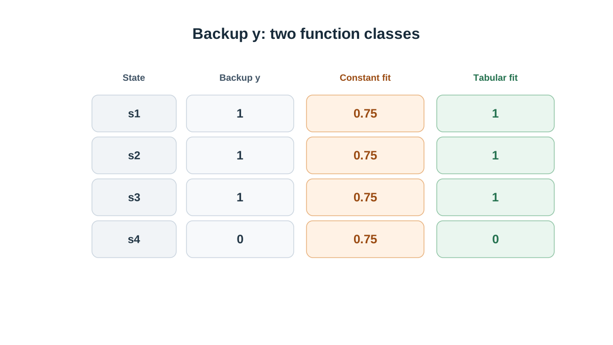
Let me make this concrete with a chain small enough to check by hand.
Four states in a line: . Fixed policy moves right. Reward is on every transition except the terminal step from , which gives . Discount .
The true values are a geometric sum:
| State | |
|---|---|
Now restrict to constant functions: for all . One parameter. This is the smallest possible restricted class, and it is exactly the kind of restriction a poorly chosen feature set creates in practice.
Start from . The Bellman backup is
With , the backup is across the four states. That vector is not constant. The backup lands outside .
Project onto the constant class by least squares. The mean of is , so everywhere. The residual is
| State | Backup | Residual | |
|---|---|---|---|
The residual is nonzero at every state, and it has opposite signs. Positive errors at through and a negative error at . If you average the squared residual, the signed errors partially cancel in the mean and the scalar loss looks smaller than the worst-case error. The pattern is exactly what a single number hides.
Contrast with tabular representation. With one parameter per state, the backup is representable exactly. The residual can be driven to zero everywhere. The restricted class cannot do that, no matter how long you train.
Note: The residual map is the diagnostic. A scalar loss is a summary; the per-state residual is the shape of the failure.
Knowledge check
Check your understanding
Answer this question before you continue.
Why a Low Training Loss Can Hide a Wrong Value Function
Now connect the decomposition back to the symptom.
The loss is an average over the sampled distribution. States that are rarely visited contribute almost nothing. Their errors are effectively invisible. In the chain example, if is visited once per episode and through are visited constantly, the loss is dominated by the three states where the residual is small.
Averaging cancels signed residuals. Large positive and negative errors at different states can sum to a small mean squared residual. The chain example shows this directly: three times and once averages to zero.
The target moves. The target is a function of the current parameters. The loss can be small at a point that is not the fixed point of the projected Bellman operator. You are chasing a target that is chasing you.
Distribution shift turns a small training loss into a large generalization gap. The data the loss is computed on and the states the policy actually visits are not the same distribution. A small training loss on one distribution says nothing about the other.
A low loss is still useful evidence that the optimizer is working and the targets are being fit. It is just not evidence about approximation error or coverage. Those are separate questions with separate answers.
Reading a Bellman-Error Number Without Being Fooled
Here is the routine I use. Ask three questions in order.
First: which distribution was the error measured under? If it does not match the states the policy visits, the number is describing the wrong problem.
Second: is the class expressive enough? If the residual is concentrated in a few states and does not shrink with more training, the class cannot represent the backup there. A richer class is the fix.
Third: did the optimizer converge? If the residual is spread evenly and shrinks with more training, you have optimization error. More steps, better learning rates, better conditioning.
Fourth: is the data covering the relevant states? If the residual is concentrated in rarely visited states, more data is the fix.
| Symptom | Likely cause | Fix |
|---|---|---|
| Residual concentrated in a few states, stable across training | Approximation error | Richer class or better features |
| Residual spread evenly, shrinking with training | Optimization error | More steps, better optimizer |
| Residual concentrated in rarely visited states | Sampling error | Better coverage |
| Residual small on training states, large on policy states | Distribution shift | Align data collection with policy |
When not to reach for this analysis: if the class contains the true value function and coverage is adequate, the approximation term is zero and the remaining work is ordinary supervised regression. Do not over-engineer a problem that is already well-posed.
What This Means for the Algorithms You Will Meet Next
Projected backups are the reason target networks, replay buffers, and residual-based objectives exist. They are attempts to control specific terms in the decomposition, not generic stabilizers. A target network slows the moving-target problem. Replay improves coverage and reduces correlation. Neither fixes approximation error.
Actor-critic critics inherit the same limits. A critic's low loss does not certify the advantage estimates the actor is trained on. The critic is a function approximator with a stated domain of validity, and that domain has to be checked against where the policy actually operates.
Treat the value function as a model with a stated domain of validity. Check that domain against where the policy operates. That is the durable habit.
Here is the concrete next step. Instrument one small value-prediction run to log the residual per state group, not just the aggregate loss. Group states by visit frequency and by region of the state space. Compare that residual map against the states the policy actually visits. If the map is flat and small everywhere the policy goes, you have earned some confidence. If it is small on average but large where the policy lives, you have found the bug the loss curve was hiding.
Knowledge check
Final check
Finish the article by checking the ideas you just learned.
References
Build a stronger RL mental model
Use structured resources to connect equations, algorithms, and observable agent behavior.


