Trace a Linear Counterexample to the Deadly Triad

Everyone repeats that the deadly triad diverges. Almost nobody watches it happen. So let's build a predictor small enough to update by hand, then watch the parameters walk away from the fixed point while the predictions barely move.

This is a trace, not a proof. We will set up a linear value predictor, train it with semi-gradient TD(0) on off-policy samples, and compute the first few updates with real numbers. By the end you should be able to point at the exact term that lets the parameters grow, and you should know precisely how much the example does and does not claim.

What We Are Actually Building

We are solving a prediction problem, not a control problem. We estimate $V(s)$, the value of a state under a fixed target policy, and we never touch policy improvement. That matters because it isolates the instability. If the parameters blow up here, no amount of action selection or exploration tuning explains it away.

The whole system is deliberately tiny: a handful of states, a linear parameter vector, one feature matrix. Small enough that you can check every number with a calculator.

I am assuming you already know the three ingredients individually — bootstrapping, function approximation, and off-policy learning — and that you have seen why a table behaves differently from a parameterized function. If that is shaky, read the triad overview and the tabular-versus-approximation comparison first; we will not re-derive them here.

The deliverable is a numeric trace of parameter updates, plus a clear statement of what the example proves and what it leaves untouched.

Notation and the Linear Prediction Setup

Define the value estimate as a linear combination of features:

$V(s; \theta) = \theta^\top \phi(s)$

where $\phi(s) \in \mathbb{R}^d$ is the feature vector for state $s$ and $\theta \in \mathbb{R}^d$ is the parameter vector we are learning. Stack the state feature vectors as rows of a matrix $\Phi$. The choice of $\Phi$ matters far more than the choice of step size in this example, and that is the whole point.

Two policies appear:

• $\mu$, the behavior policy, which generates the transitions we actually observe.
• $\pi$, the target policy, whose value function we want to estimate.

They differ. That difference is the off-policy ingredient, and it is not cosmetic — it changes which states get visited and how often.

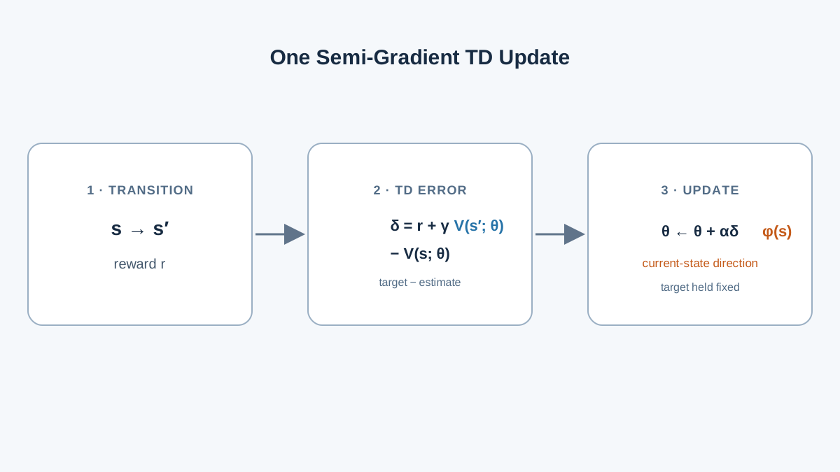
Fix a discount factor $\gamma \in [0, 1)$ and a step size $\alpha > 0$. For a sampled transition $(s, r, s')$, the TD error is:

$\delta = r + \gamma V(s'; \theta) - V(s; \theta)$

The update rule is:

$\theta \leftarrow \theta + \alpha \, \delta \, \nabla_\theta V(s; \theta)$

Since $V(s; \theta) = \theta^\top \phi(s)$, the gradient is just $\phi(s)$. So the update becomes:

$\theta \leftarrow \theta + \alpha \, \delta \, \phi(s)$

Look closely at that gradient. It is taken only on the current estimate $V(s; \theta)$, not on the bootstrapped target $r + \gamma V(s'; \theta)$. The target also depends on $\theta$, but we ignore its derivative. That single omission is the semi-gradient move, and it is where the trouble lives.

Why the Feature Matrix Is the Trap

Here is the structural condition that makes this example diverge, and it is worth understanding before any arithmetic.

The feature vectors are arranged so that the parameter vector can grow while the represented value function stays nearly unchanged. In other words, there is a direction in parameter space along which $\Phi \theta$ is almost constant. The data does not pin the parameters down; it only pins down the predictions.

Under on-policy sampling, the state distribution would weight updates so that this loose direction gets damped. Under off-policy sampling, the states that would correct the growing direction are visited less often than the states that amplify it. The correction never arrives.

Contrast this with a table. In a tabular representation, each state owns its own parameter. There is no shared direction for error to accumulate along, because no two states write to the same number. Function approximation couples states through shared weights, and off-policy sampling changes which couplings actually get corrected. That coupling is the hidden constraint worth remembering.

Tracing the First Updates by Hand

Now the numbers. I will use a compact version of the classic Baird-style construction: a set of states whose feature vectors share a common component, with a behavior policy that over-samples the states pushing the shared component up.

Set $\gamma = 0.99$ and $\alpha = 0.1$. Initialize every parameter to $1$. Suppose we have two states of interest with feature vectors:

$\phi(s_1) = [2, 0, 1]^\top, \qquad \phi(s_6) = [0, 2, 1]^\top$

With $\theta = [1, 1, 1]^\top$:

$V(s_1) = 2(1) + 0(1) + 1(1) = 3$ $V(s_6) = 0(1) + 2(1) + 1(1) = 3$

First transition: $s_1 \to s_6$ with reward $r = 0$.

$\delta = 0 + 0.99 \cdot 3 - 3 = -0.03$

The gradient with respect to $\theta$ is $\phi(s_1) = [2, 0, 1]^\top$. Apply the update:

$\theta \leftarrow [1, 1, 1]^\top + 0.1 \cdot (-0.03) \cdot [2, 0, 1]^\top = [0.994, 1, 0.997]^\top$

Small correction. Fine.

Second transition: now suppose the behavior policy feeds us $s_6 \to s_6$ with reward $r = 0$, a self-loop that the target policy would rarely take.

$V(s_6) = 0(0.994) + 2(1) + 1(0.997) = 2.997$

$\delta = 0 + 0.99 \cdot 2.997 - 2.997 = -0.02997$

Update with $\phi(s_6) = [0, 2, 1]^\top$:

$\theta \leftarrow [0.994, 1, 0.997]^\top + 0.1 \cdot (-0.02997) \cdot [0, 2, 1]^\top = [0.994, 0.994, 0.994]^\top$

Notice what happened. The parameters moved together, and the value estimates barely budged — $V(s_1)$ is still about $2.98$. The predictions are stable-looking. The parameters are not converging to anything meaningful; they are sliding along the loose direction I described earlier.

If you keep feeding self-loops and shared-feature transitions under this behavior policy, the shared component keeps absorbing updates. The norm of $\theta$ climbs. The predictions drift slowly. The divergence lives in the parameters first.

Note: This is why watching the loss alone can fool you. A nearly flat value-error curve can hide a parameter vector that is quietly growing without bound.

Why the Updates Keep Growing

Connect the arithmetic back to the mechanism.

The target $r + \gamma V(s'; \theta)$ is built from the same $\theta$ being updated. An error in $\theta$ becomes part of the next target, which produces the next error. That is the bootstrapping feedback loop: the estimate feeds itself.

Because the behavior policy $\mu$ differs from the target policy $\pi$, the states that would pull the shared component back down are under-visited. The states that push it up are over-visited. Off-policy sampling keeps feeding the unstable direction.

And the semi-gradient ignores the derivative of the target. There is no term in the update that pulls the parameters back toward a fixed point. The update has no restoring force.

Compare tabular TD with on-policy sampling. There, the update is a contraction: each state's estimate moves toward a target that depends on other states' estimates, and the whole system contracts toward a reachable fixed point. Remove the table and the on-policy distribution, and the contraction argument no longer holds.

What This Example Does Not Prove

Bound the claim before you over-generalize.

Divergence here is a property of this update rule under these assumptions. It is not a universal law that all function-approximation RL diverges. Plenty of function-approximation methods converge under the right conditions.

This is a prediction problem with a fixed policy. It says nothing directly about control algorithms, and nothing about deep networks that carry stabilization machinery this example lacks — target networks, regularization, replay with bounded targets, or on-policy data collection.

Practical systems often stay stable precisely because of those mechanisms. The correct reading is a warning about assumptions, not a verdict on function approximation.

How to Use This as a Debugging Lens

Turn the theory into a diagnostic you can run.

When value estimates blow up, check the three ingredients in order:

1. Is the target bootstrapped? If you replaced it with a Monte Carlo return, does the instability vanish?
2. Is the representation shared across states? If you switch to a table for a small version of the problem, does it stabilize?
3. Is the data off-policy? If you collect on-policy, does the growth stop?

Watch the parameter norm, not just the loss. A stable-looking loss can hide a growing parameter vector, as the trace above showed.

If you can switch to on-policy data or a tabular representation for a small version of the problem, do it and see whether the instability disappears. That isolates the cause instead of guessing. And evaluate across repeated runs and learning curves rather than trusting a single trajectory — one lucky seed can mask a structural problem.

The next step is concrete: reproduce this trace in a few lines of code, then deliberately remove one ingredient — make the sampling on-policy, or replace the shared features with a table — and watch the behavior change. When you see divergence in your own experiments, do not assume a bug. First ask which of the three ingredients is present, and whether your representation gives the parameters room to grow without changing the predictions.