
Generalization in Reinforcement Learning: Task Distributions and the Generalization Gap
A policy scores well on a handful of held-out levels. The write-up says it "generalizes to unseen environments." Then deployment happens, and the policy…

Key topics
A policy scores well on a handful of held-out levels. The write-up says it "generalizes to unseen environments." Then deployment happens, and the policy falls apart on the first environment that was not in that handful. Nothing was falsified. Nothing was even wrong, exactly. The claim was just never specific enough to be checked.
That is the failure I want to fix here. Generalization in reinforcement learning is not a property a policy carries around like a passport stamp. It is a relation between a policy and a distribution of tasks. Name the distribution, and the claim becomes measurable. Leave it out, and you have a number that means whatever the reader wants it to mean.
This builds on the evaluation habits you already have: repeated episodes, multiple seeds, held-out variations. Those tell you about variance. They do not tell you which distribution you sampled from, and that is the gap this article closes.
Why "It Generalizes" Is an Incomplete Claim
Two teams can report the same held-out mean and be making completely different claims. One tested on levels drawn from the same generator that produced training levels. The other tested on levels from a different generator with different physics. Same number, different universe.
The missing piece is always the same: the distribution. A policy is only ever good at something, and that something is a set of tasks with a sampling rule. When the rule is implicit, the claim cannot be audited, reproduced, or falsified. A reviewer cannot ask "did you cover the friction range you claim to cover?" because no range was ever written down.
Here is the reframe I want you to carry through the rest of this article:
Note: Generalization is a property of the pair (policy, task distribution), not of the policy alone. Change the distribution and you have changed the claim.
Tasks as Samples: The Distribution You Actually Trained On
Let me put notation on the table before using it.
A task (sometimes called a context) is a single instance of the problem: one level, one physics configuration, one target position. Write it as . Tasks are drawn from a distribution . A policy is , and is a performance measure in task — usually expected return, but it could be success rate or time-to-goal.
Training does not optimize against . It optimizes against a finite sample:
That distinction matters more than it looks. A narrow makes the training objective a poor proxy for anything wider, and a small means you may not have seen much of either. You can have a wide distribution and still overfit to a thin slice of it.
The distribution itself is usually parameterizable, and naming the parameterization is most of the work:
| Task family | What the distribution parameterizes |
|---|---|
| Procedural levels | Random seed for the level generator |
| Sim-to-real robotics | Physics parameter vector (friction, mass, latency) |
| Manipulation benchmarks | Task id from a fixed set |
| Control suites | Target position or goal region |
Common mistake: Treating the training set as the training distribution. The set is a sample. If you trained on 50 seeds from a generator that can produce millions, your policy saw 50 points, not the generator.
Knowledge check
Check your understanding
Answer this question before you continue.
Defining the Generalization Gap
Now the quantity that makes the claim checkable. Expected performance on a distribution is:
The generalization gap is the difference between expected performance on the training distribution and expected performance on an evaluation distribution:
This is a population quantity: it compares two distributions, not two samples. When you compute it in practice, you replace each expectation with a sample mean, and the result is an estimate of the gap, not the gap itself. Keep that distinction in your head, because it is exactly where most reporting goes wrong.
A related but distinct quantity is per-task regret: how far the policy sits from the best possible policy for each task, averaged over the evaluation distribution.
where is the best policy for task . Regret answers "how much performance did we leave on the table per task?" The gap answers "how much did performance change when we moved from one distribution to another?" They are different questions, and I will use the gap — not regret — for the worked example below.
Three assumptions are baked into the gap, and each one can fail:
- The evaluation tasks are drawn from the distribution you claim. If they are not, you are estimating a gap for a different distribution than the one in your write-up.
- The sample is large enough to estimate the expectation. A gap computed from three tasks is a noisy estimate of the gap, not the gap.
- is measured the same way in training and evaluation. Different episode limits, different reward clipping, different termination rules — any of these silently changes what you are comparing.
Knowledge check
Check your understanding
Answer this question before you continue.
Worked Example: Two Protocols, Two Different Failures
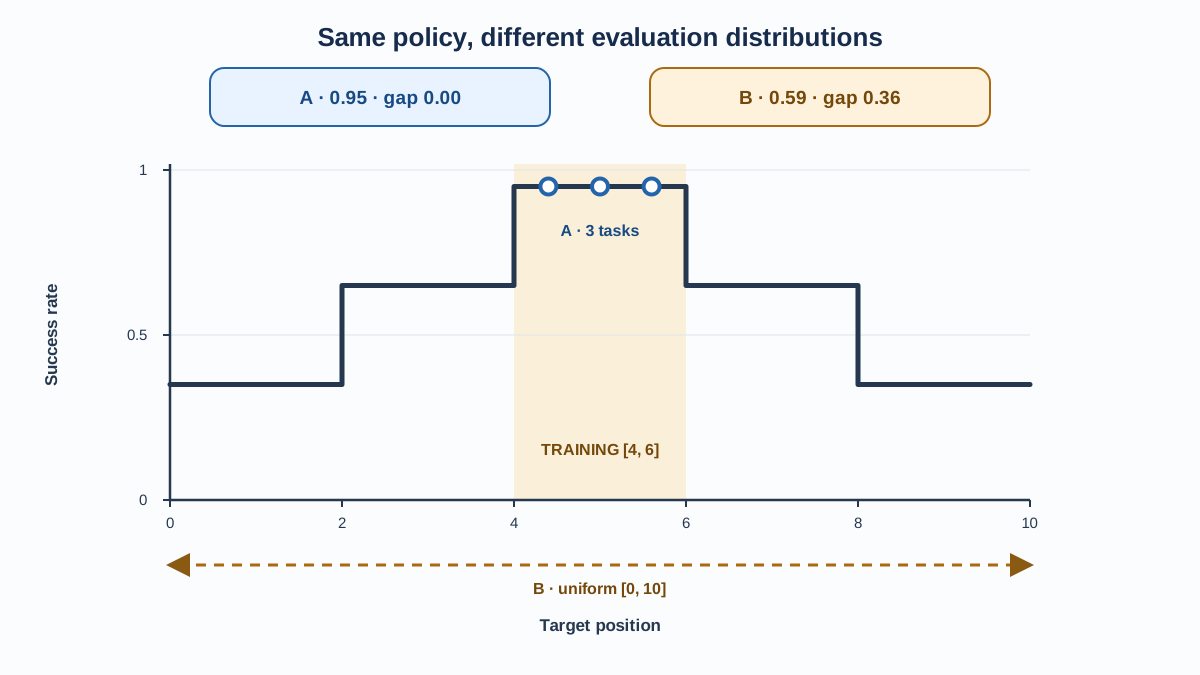
Take a small task family with one varying parameter: a target position on a line, with . The policy is trained on tasks sampled from — a narrow slice. Performance is success rate, and suppose it looks like this:
- : success rate 0.95
- : success rate 0.70
- : success rate 0.30
Now run two evaluation protocols and see what each one can actually support.
Protocol A — same distribution, small sample. Evaluate on three tasks at . All three are inside the training range, and they are drawn from the same . Sample mean: 0.95. Estimated gap: 0.00.
This protocol is not meaningless. It is a valid held-out estimate of same-distribution generalization — performance on fresh tasks from the training distribution. What it cannot do is support a claim about anything outside . The three-task sample is also too small to trust on its own; a lucky draw of three easy positions looks identical to a policy that truly handles the whole range.
Protocol B — genuinely shifted distribution. Evaluate on tasks drawn uniformly from . This is a different distribution from , so the estimated gap now measures distribution shift. Expected performance is roughly:
Estimated gap: . Now the number is a claim about a stated distribution, and it is large enough to matter.
The two protocols fail in different ways. Protocol A answers a narrow question correctly and gets over-claimed as if it answered a wide one. Protocol B answers the wide question and reveals the cliff. Neither is a bug in the math. The bug is in the sentence that follows the number.
Tip: Plot per-task performance against the task parameter, shade the training range, and mark the evaluation samples. The gap becomes an area you can see, not a number you have to trust.
Knowledge check
Check your understanding
Answer this question before you continue.
What Held-Out Estimates Can and Cannot Tell You
A held-out estimate is an estimate of expected performance on the distribution you sampled from. That is the entire content of the number. It cannot tell you about tasks outside that distribution, and it degrades silently as the evaluation distribution drifts from the deployment distribution — silently because nothing in the number itself signals the drift.
Sample size and coverage are separate axes. Many tasks from a narrow distribution still cannot support a wide claim. A few tasks from a wide distribution support a wide claim weakly. You need both, and you need to say which one you have.
The decision rule I use before writing any transfer claim:
- Write down — the parameterization and the range.
- Write down — the parameterization, the range, and the sample size.
- Write down the deployment distribution you actually care about.
- Compare to deployment. Where does evaluation not reach?
If step 4 has an answer, the claim needs to be scoped to match.
Warning: When training and deployment genuinely share one fixed environment, this framing adds ceremony without adding information. If there is no distribution — one environment, one deployment — say so and move on.
Knowledge check
Check your understanding
Answer this question before you continue.
Reporting a Generalization Result You Can Defend
The theory collapses into a short checklist. Apply it to your next write-up:
- Name the task distribution and how tasks were sampled from it, including the parameterization and range.
- Report the number of training and evaluation tasks. Both, not just evaluation.
- Report per-task spread, not only the mean. The variance across tasks is where the interesting information lives.
- State the deployment distribution the claim is meant to cover, and say explicitly where evaluation does not reach it.
- Flag the gap as an estimate with uncertainty, not a fixed property of the policy.
The most common mistake is reporting a single held-out mean and calling it generalization. A mean of 0.94 across ten tasks that range from 0.30 to 0.95 tells a very different story than a mean of 0.94 across ten tasks that all sit near 0.94. The first policy has a cliff. The second does not. The mean hides the cliff.
Where This Leaves You
Go back to the opening scene. The same held-out score is now readable as a claim about a specific distribution with specific limits — or as a claim that was never specific enough to check. The difference is not the number. It is whether you wrote down what the number was a number about.
Before you run anything else, write three lines: , , and the deployment distribution you actually care about. If you cannot fill in the third line, you do not yet have a transfer claim — you have a benchmark result.
The next question is the one this framing sets up but does not answer: how do you design task variations that probe a reusable strategy rather than memorized specifics? That is a design problem, and it deserves its own experiment.
Knowledge check
Final check
Finish the article by checking the ideas you just learned.
References
Build a stronger RL mental model
Use structured resources to connect equations, algorithms, and observable agent behavior.


