
Uncertainty in Reinforcement Learning Evaluation: Comparing Runs and Policies
Two algorithms. Five seeds each. A forty-point gap in mean return. Someone asks which one to ship, and the honest answer is: you do not know yet. Not…

Key topics
Two algorithms. Five seeds each. A forty-point gap in mean return. Someone asks which one to ship, and the honest answer is: you do not know yet. Not because the experiment was sloppy, but because a mean is a sample, not a verdict.
Here is the weak model underneath most RL comparisons: the mean is the result. It is not. The mean is one draw from a distribution of possible experiments, and the real question is how much of that forty-point gap survives resampling. Answering that question requires three things — a named target quantity, an interval, and a decision about pairing.
What You Are Actually Estimating
Before you compute anything, name the quantity you want to estimate. This is the estimand, and getting it wrong is the most common source of bad comparisons.
Two estimands show up constantly in RL evaluation, and they are not interchangeable:
- Expected return of a fixed policy under a fixed evaluation protocol. You have one trained policy, and you want to know how well it performs. The randomness here comes from the environment and the policy's own stochasticity.
- Expected performance of a training procedure across seeds. You have an algorithm, and you want to know how well it performs when you run it again from scratch. The randomness here includes everything in the first estimand plus the seed-to-seed variation in training.
These demand different uncertainty treatment. If you trained one policy and evaluated it on a thousand episodes, a tight interval around its mean return tells you about evaluation noise — not about whether the algorithm is reliable. If you trained five policies from five seeds and averaged their returns, your interval speaks to the training procedure, but only if you treat seeds as draws from a population of possible runs.
Three sources of variation feed into any number you report:
- Within-episode stochasticity — the environment and policy are random, so two episodes from the same policy differ.
- Seed-to-seed training variability — different initializations, data orderings, and exploration trajectories produce genuinely different policies.
- Evaluation-sampling noise — you tested on a finite number of episodes, so your estimate of any single policy's return is itself uncertain.
The sampling assumption is blunt: seeds are draws from a population of training runs, and episodes are draws from the environment's return distribution. If either assumption is shaky — say, you hand-picked seeds that happened to work — the interval you compute is decorative.
If you have already built evaluation around repeated episodes and seeds, you have the raw material. This article is about what those numbers can support as a claim.
Knowledge check
Check your understanding
Answer this question before you continue.
Run-to-Run Variability Is Not the Same as Uncertainty
A wide spread across seeds is a property of the algorithm. The standard error of the mean is a property of your sample size. These are separate facts, and conflating them leads to bad decisions.
Run-to-run variability is the spread of the seed-level distribution — the thing you see in a seed plot or a min/max band. It tells you how much the algorithm's outcome depends on the seed.
Uncertainty in the sample mean is how precisely you have pinned down the center of that distribution. It shrinks roughly with the square root of the number of seeds.
Consider five seeds with returns of 120, 340, 210, 90, and 240. The mean is 200. The standard deviation is about 102. The standard error is 102 / √5 ≈ 46. So your interval around the mean is roughly ±90 at 95% confidence — wide enough that a forty-point gap between two algorithms means almost nothing.
Now imagine the same spread across twenty seeds. The standard error becomes 102 / √20 ≈ 23, and the interval narrows to roughly ±45. The dots on the seed plot have not moved. The algorithm is exactly as variable as it was. You have only bought precision about where the center sits.
Common mistake: Reporting a narrow interval around the mean and concluding the algorithm is "stable." Stability is the spread of the dots. Precision is the width of the interval around their center. Both belong in the report.
Knowledge check
Check your understanding
Answer this question before you continue.
Building an Interval You Can Defend
The standard error of the mean comes from the seed-level standard deviation and the number of seeds :
The denominator is because averaging independent draws reduces the variance of the mean by a factor of , and the standard deviation by . That is the whole mechanism.
With five to ten seeds, the normal approximation is optimistic. The sample standard deviation is itself noisy, so a -based interval is the more defensible default:
For , rather than the normal . That difference is not cosmetic — it is the interval admitting it does not know the spread very well yet.
When the closed form does not apply — medians, interquartile ranges, aggregate scores across tasks — use the bootstrap. Resample the seed-level scores with replacement, recompute the mean, repeat a few thousand times, and take the 2.5th and 97.5th percentiles of the resampled means. The idea is one paragraph long and generalizes to almost any aggregate you care about.
The assumptions are worth stating plainly:
- Seeds are independent.
- The seed-level distribution is roughly stable across the sample.
- You did not cherry-pick which seeds entered the sample.
That last one invalidates the interval regardless of method. If you tuned on seeds 1–5 and reported on seeds 1–5, the interval describes a search, not an experiment.
There is also a practical ceiling. More seeds reduce statistical uncertainty but cost compute. The honest move is to report the interval you actually bought, not to imply precision you did not pay for.
Knowledge check
Check your understanding
Answer this question before you continue.
Paired vs Unpaired Comparisons
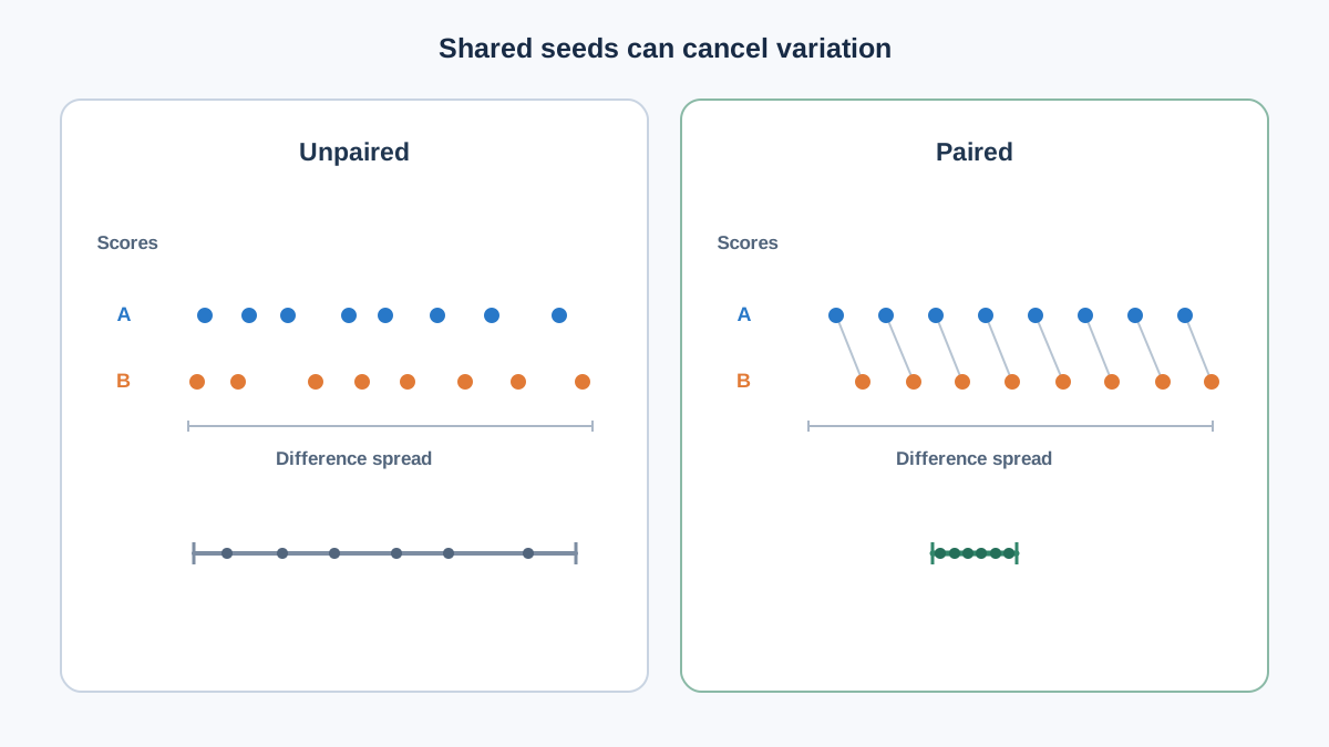
The same five seeds can make a difference far more credible — if you pair them.
The paired estimand is the expected difference in return between two policies evaluated under the same seed, environment instance, or evaluation episode set. Pairing removes the shared component of variation. The standard error of the difference then depends on the variance of the per-seed differences, not on the sum of two independent variances.
Suppose Algorithm A returns 120, 340, 210, 90, 240 and Algorithm B returns 100, 310, 190, 70, 220 on the same five seeds. The per-seed differences are 20, 30, 20, 20, 20. The mean difference is 22, and the standard deviation of the differences is about 4.5. The paired standard error is 4.5 / √5 ≈ 2. That is a tight interval around a consistent positive difference.
Now compute the unpaired interval from the same numbers. Algorithm B's standard deviation is about 97, so the unpaired standard error of the difference is roughly √(46² + 43²) ≈ 63. The same data now produces an interval so wide it cannot distinguish the algorithms.
| Aspect | Paired | Unpaired |
|---|---|---|
| Assumption | Seeds control something shared | Runs are independent draws |
| Variance source | Variance of per-seed differences | Sum of two independent variances |
| Typical reduction | Large when seed effects dominate | None |
| Right call | Same seed, environment instance, or eval episodes | Runs cannot share control |
Warning: A post-hoc seed match is not a true pairing. If seed 3 for Algorithm A and seed 3 for Algorithm B were not run under the same initialization, environment instance, and evaluation episodes, you have not removed the shared variation — you have only relabeled it.
The decision rule is short: pair whenever the seed controls something shared. Do not pair when the two runs cannot share that control, and do not pretend a coincidental index match is a pairing.
Knowledge check
Check your understanding
Answer this question before you continue.
When the Interval Says Nothing Useful
A correct interval can still mislead. These are the failure modes I see most often.
Overlapping intervals. Two separate intervals overlapping does not mean the difference is zero, and non-overlapping intervals do not guarantee a real difference. The interval for a difference is not the visual gap between two intervals. Compute the difference directly.
Selection effects. Tuning on the same seeds you later report, or reporting the best checkpoint, converts a valid interval into a biased one. The interval assumes the sample was drawn, not chosen.
Aggregation traps. Averaging across tasks with different score scales can hide per-task reversals. Report the aggregate and the per-task picture together.
Heavy-tailed returns. When the distribution is skewed, the clean standard-error story breaks. Prefer bootstrap intervals and report the distribution rather than only the center.
Too few seeds. With two or three seeds, an interval is a costume, not evidence. Say so and run more seeds, or narrow the claim to a qualitative observation.
Reporting the Comparison Without Overclaiming
Turn the machinery into a short, honest reporting pattern.
Report the estimand, the number of seeds, the interval method, and the pairing structure in one compact block. A reader should be able to reconstruct the claim without guessing.
Prefer a stated interval over a significance verdict. An interval carries magnitude and uncertainty; a binary significant/not-significant label throws away both. Show the seed-level distribution alongside the summary, because the spread is often more decision-relevant than the mean.
Precommit to the comparison before running final seeds. The interval should describe a planned test, not a search for a favorable result.
The practical consequence: a difference that survives pairing and a defensible interval is worth acting on. A difference that exists only in point estimates is a hypothesis, not a finding.
Before you claim one policy beats another, name the estimand, state the pairing, and report an interval. Then act only on differences that survive all three. If you already have a comparison sitting in a notebook, the next step is to rerun it with paired seeds and an interval attached. When the interval comes back wide and the cause is unclear, the diagnostic and ablation material in this category is where to look next.
Knowledge check
Final check
Finish the article by checking the ideas you just learned.
References
Build a stronger RL mental model
Use structured resources to connect equations, algorithms, and observable agent behavior.


