
Derive Log Probabilities for Squashed Continuous Actions
A SAC actor hands you two tensors: the action you just sent to the environment, and logp_pi. That second number is not the Gaussian log-density of the…

Key topics
A SAC actor hands you two tensors: the action you just sent to the environment, and logp_pi. That second number is not the Gaussian log-density of the action. It is the Gaussian log-density of the action after a transform moved the probability mass around — and if you forget the correction, your likelihood-ratio term quietly optimizes a distribution the environment never sees.
This is the derivation behind that correction. It is short, it is one-dimensional, and once you have it you can read the log-probability line in any squashed-policy implementation and predict where it breaks.
Why the Sampled Action's Density Is Not the Gaussian's Density
Continuous-control actors parameterize a factored Gaussian over a pre-squash variable . The environment, however, receives
so the behavior distribution lives on , not on the real line. The network's parameters describe ; the environment experiences . Those are different objects.
The policy-gradient estimator needs for the action actually taken. If you substitute for , you are scoring a different event. The update is no longer an unbiased estimate of the gradient of the objective you think you are optimizing.
Two failure modes follow from that substitution:
- The density is wrong, and it is wrong unevenly. Near the bounds, the gap between the naive Gaussian density and the true squashed density is largest — exactly where trained continuous-control policies spend most of their time.
- The gradient path ignores how the transform compresses the action axis. The reparameterized sample flows through , and the likelihood term must account for that compression or the policy receives a distorted learning signal.
I am assuming you already accept the likelihood-ratio form of the policy gradient and the reparameterized sample. Both are covered elsewhere in this curriculum. What matters here is the density correction that sits between them.
Prerequisites: Bijective Maps and the One-Dimensional Change-of-Variables Rule
A change of variables requires a bijection between supports. is a strictly increasing bijection from onto . That is the entire reason the rule applies — and the reason clipping cannot use it.
For a monotone transform with inverse ,
The absolute value matters because densities are non-negative; the derivative of an inverse can be negative for a decreasing transform, and the sign is not part of the density.
Read the Jacobian factor as a local volume correction. Where the transform stretches the axis, density thins out. Where it compresses the axis, density piles up. The total probability is preserved; the shape is not.
Common mistake: treating a hard clamp as a change of variables. A clamp is not injective — many values map to the same boundary action — so it has no inverse and no Jacobian. You cannot correct a clamp this way. That distinction is the whole comparison in the last section.
Knowledge check
Check your understanding
Answer this question before you continue.
Deriving the Squashed Density for
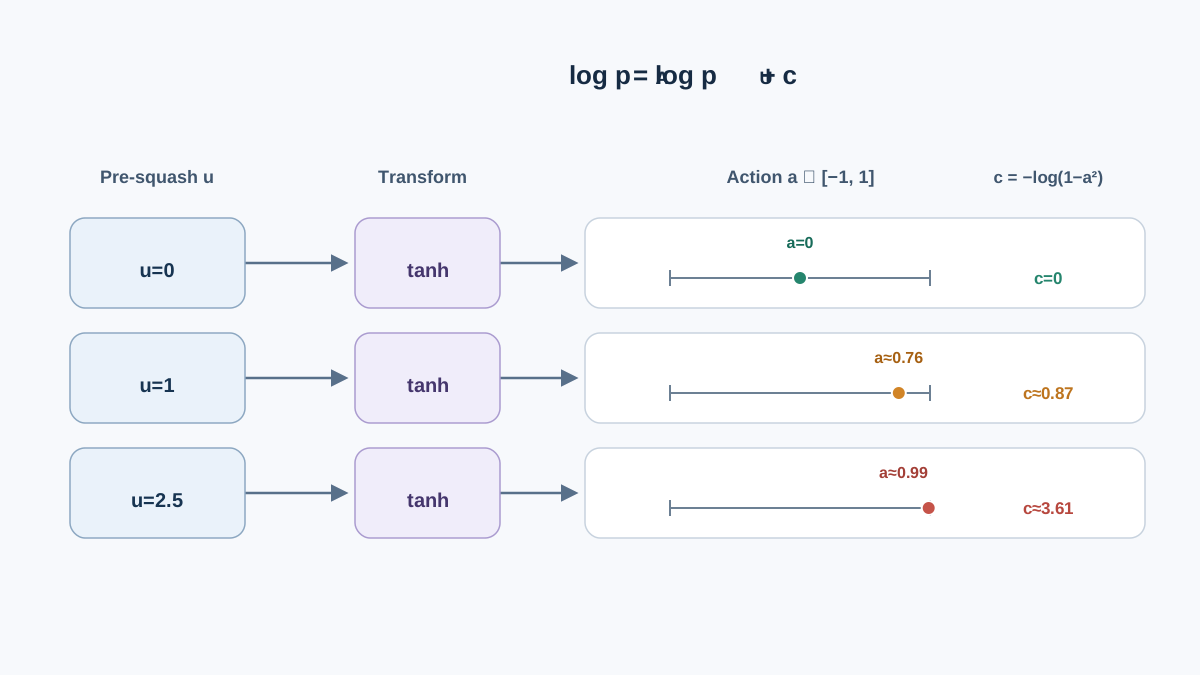
Set the notation. Let
with the Gaussian density and the density of the squashed action. The inverse is
Differentiate the inverse with respect to :
In one dimension, that derivative is the Jacobian. Assemble the density:
Take logs:
That is the squashed Gaussian policy log probability in one line. The correction term is .
Two things to notice about the sign. The correction is subtracted, so the squashed density is always smaller than the naive Gaussian density evaluated at the same point. And the gap widens as , because and . The transform does not merely clip the tails; it redistributes their mass inward and charges you a log-density penalty for standing near the edge.
For multi-dimensional actions, the transform is applied per dimension and the Jacobian is diagonal, so the log-determinant is just the sum of the per-dimension corrections:
No cross terms, because the transform does not mix dimensions.
Knowledge check
Check your understanding
Answer this question before you continue.
Worked Example: One Action, Two Densities
Numbers make this concrete. Take , , and sample .
The Gaussian log-density at :
The correction term:
So the corrected log-density is
Now push toward the bound. Sample :
The Gaussian log-density at is roughly , so the corrected value is about . The correction has grown from to — a factor of four — while the action moved only from to .
And at : , , and the correction is exactly zero. Near the center of the action range, squashing is locally the identity and the naive density is correct. The error is a boundary phenomenon.
The observable consequence: an uncorrected implementation understates the likelihood of near-boundary actions. Since trained policies concentrate their mass near the limits of the useful range, that understatement is not a corner case. It is the operating regime.
You can verify the arithmetic directly:
import numpy as np

def squashed_log_prob(u, mu=0.0, sigma=1.0):
    a = np.tanh(u)
    gaussian_logp = -0.5 * np.log(2 * np.pi * sigma**2) - 0.5 * ((u - mu) / sigma) ** 2
    correction = -np.log(1 - a**2)
    return gaussian_logp, correction, gaussian_logp + correction

for u in [0.0, 1.0, 2.5]:
    naive, corr, corrected = squashed_log_prob(u)
    print(f"u={u:>4}  naive={naive: .4f}  correction={corr: .4f}  corrected={corrected: .4f}")
Run it. Watch the correction column stay at zero for the centered sample and climb for the boundary sample. That column is the entire derivation.
Knowledge check
Check your understanding
Answer this question before you continue.
Squashing Versus Clipping: Two Different Ways to Break a Density
Clipping and squashing both produce bounded actions. They are not interchangeable, and the difference is structural, not stylistic.
Clipping maps an entire interval of values onto a single boundary action. Every becomes . The result is not a density on the action space at all — it has an atom of probability mass at each bound. Total probability is still one, but it is no longer spread continuously across the support.
Squashing is a bijection. Nothing collapses. Total probability is preserved, and is a genuine density everywhere on . The shape changes; the validity does not.
| Property | Squashing () | Clipping |
|---|---|---|
| Map type | Bijective | Many-to-one |
| Support | with atoms at bounds | |
| Density valid everywhere | Yes | No — atoms at the limits |
| Likelihood-ratio term | Valid after Jacobian correction | Biased by boundary effect |
| Typical failure symptom | Correction diverges near bounds | Policy slams into limits |
The gradient consequence follows from the table. Under squashing, the likelihood-ratio term stays valid once you apply the correction. Under clipping, the estimator integrates over a support the policy does not actually cover, which introduces a boundary bias: the gradient treats boundary actions as if they were sampled from the interior density, when in reality they were piled up by the clamp.
The exploration consequence is visible in the action histogram. When the Gaussian's spread is wide relative to the action range, clipping oversamples the bounds. The policy looks like it keeps slamming into its limits — because it does.
Knowledge check
Check your understanding
Answer this question before you continue.
When the Correction Matters, and When It Is Overkill
Squashing earns its cost when the policy must be stochastic and bounded, and when the likelihood-ratio or entropy term is part of the objective. SAC-style setups are the canonical case: the entropy term depends on , so an uncorrected density corrupts the entropy estimate as well as the policy gradient.
Clipping is defensible when the action range is wide relative to the policy's spread. If almost no probability mass reaches the bounds, the boundary bias is negligible and the simpler parameterization is fine. The decision boundary is the ratio of policy spread to action range — not a matter of taste.
Neither is the right answer when the action distribution is genuinely bounded and non-Gaussian in shape. A distribution with native bounded support, such as a Beta policy, avoids the transform entirely and needs no Jacobian correction.
Warning: the correction diverges as . Implementations need a small epsilon inside the log — something like
-torch.log(1 - a**2 + 1e-6)— to avoid infinities during early training when the policy is still exploring the full range.
My diagnostic rule: if actions cluster at the limits and the entropy term behaves strangely, suspect the interaction between the transform and the action range before you blame the optimizer. The density correction is the first place to look, and it is cheap to check.
Reading the Correction in the Wild
The next time you open a continuous-control actor, find the line that computes logp_pi. You should now be able to point at the Jacobian correction, identify it as , and say what happens to it as the action approaches the bound: it grows without limit, and any implementation that omits it understates the likelihood of exactly the actions your policy produces most.
Two concrete next steps. First, recompute the worked example with and again with . Watch how the correction's contribution changes with the policy's spread — that is the same ratio that decides whether clipping would have been acceptable. Second, instrument an existing actor to log both the naive Gaussian density and the corrected density on every step, then plot them against the action value. The two curves will agree at the center and diverge at the edges. That divergence is the boundary effect, and seeing it once will make you check for it every time.
Knowledge check
Final check
Finish the article by checking the ideas you just learned.
References
Build a stronger RL mental model
Use structured resources to connect equations, algorithms, and observable agent behavior.


