Observe Bellman Contraction With Two Value Estimates

Two guesses walk into the same operator. One is all zeros. One is absurdly large. If the Bellman operator really is a contraction, their distance should shrink on every sweep — and never by more than the discount factor.

You have seen the claim written down: the Bellman operator is a gamma-contraction. Maybe you have even written a value-iteration loop that converges and printed a shrinking error. But watching one estimate settle down is not the same as watching two estimates get pulled together. The contraction property is a promise about the distance between any two value vectors, and the fastest way to trust it is to start two vectors far apart, apply the same operator to both, and measure the gap after each sweep.

That is the whole exercise. Same operator, different starting guesses, converging distance.

What You Are About to Prove

Before any code runs, let's name the two objects involved.

The Bellman operator takes a value vector in and returns a new value vector out. One application is one backup: for each state, look at the reward plus the discounted value of wherever you might land next. Applying it over and over is exactly what value iteration does.

The distance measure is the sup norm — the single largest absolute difference across all states. Not an average. Not a sum. The worst state wins. If you have two value vectors V and U, their sup-norm distance is max(|V[s] - U[s]|) over every state s.

The claim under test is short:

After one application of the Bellman operator, the sup-norm distance between two value vectors shrinks by at most the discount factor gamma.

In symbols: ||T(V) - T(U)||∞ ≤ γ · ||V - U||∞.

Why two vectors instead of one? Because convergence to a fixed point is really a statement about any two starting points being pulled together. If every pair of estimates gets closer, the limit has to be unique — there is nowhere else for them to go.

The Tiny MDP and the Two Starting Guesses

We need a small environment with a known model. The operator needs transition probabilities and rewards, not samples, so a hand-built tabular MDP is perfect.

Here is the setup: four states in a line, 0 through 3. From any state you can go left or right. State 3 is an absorbing terminal state: stepping into it pays a reward of 1.0, and once you are there, the episode is over — no further reward, no further continuation. Every other transition pays 0.0. If you try to step off either end, you stay put.

The discount factor is gamma = 0.9. It sits strictly between 0 and 1, which is exactly the condition the bound requires. At gamma = 1.0 the guarantee falls apart, and we will see that later.

Now the two starting guesses:

• V_zero: all zeros. The lazy guess.
• V_big: large arbitrary values, say [100, -50, 200, 10]. The confident-but-wrong guess.

The initial gap is easy to see: the largest absolute difference is 200. That is our starting distance, and every sweep should cut it down.

Run the Script

Standard library only. No installs, no credentials, no external services. Save this as bellman_contraction.py and run it.

GAMMA = 0.9
STATES = [0, 1, 2, 3]
TERMINAL = 3
REWARD = {3: 1.0}

def transitions(s, a):
    """Return list of (next_state, probability) for state s, action a."""
    if s == TERMINAL:
        return [(s, 1.0)]
    nxt = s + a
    if nxt < 0 or nxt > 3:
        nxt = s  # bounce off the wall
    return [(nxt, 1.0)]

def bellman_backup(V):
    """One application of the Bellman optimality operator."""
    new_V = {}
    for s in STATES:
        if s == TERMINAL:
            # Absorbing terminal: value is the terminal reward, no continuation.
            new_V[s] = REWARD[s]
            continue
        best = float("-inf")
        for a in (-1, +1):
            q = 0.0
            for nxt, p in transitions(s, a):
                if nxt == TERMINAL:
                    # Entering terminal pays reward, then the episode ends.
                    q += p * REWARD[nxt]
                else:
                    q += p * (0.0 + GAMMA * V[nxt])
            best = max(best, q)
        new_V[s] = best
    return new_V

def sup_norm(V, U):
    return max(abs(V[s] - U[s]) for s in STATES)

V_zero = {s: 0.0 for s in STATES}
V_big  = {0: 100.0, 1: -50.0, 2: 200.0, 3: 10.0}

prev = sup_norm(V_zero, V_big)
print(f"{'sweep':>5} {'distance':>12} {'ratio':>8}")
print(f"{0:>5} {prev:>12.6f} {'-':>8}")

for k in range(1, 21):
    V_zero = bellman_backup(V_zero)
    V_big  = bellman_backup(V_big)
    d = sup_norm(V_zero, V_big)
    ratio = d / prev if prev > 0 else 0.0
    print(f"{k:>5} {d:>12.6f} {ratio:>8.4f}")
    prev = d

The key detail is the terminal convention. Entering state 3 pays 1.0 and stops — the backup does not add GAMMA * V[3] after that reward. The terminal state's own value is pinned to 1.0 and never updated. Get this wrong and the numbers will not match what follows.

Run it and you should see:

sweep     distance    ratio
    0   200.000000        -
    1   180.000000   0.9000
    2   162.000000   0.9000
    3   145.800000   0.9000
    4   131.220000   0.9000
    5   118.098000   0.9000
    ...

The success criterion is simple: the ratio column never exceeds gamma. Here it lands exactly on 0.9 every sweep, which is the tightest case the bound allows. In messier MDPs it will often be smaller.

Read the Output Like Evidence

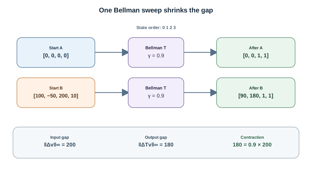
Do not just watch the numbers get smaller. Read the ratio column as a measurement.

Column	What it tells you
distance	The sup-norm gap between the two value vectors after this sweep.
ratio	This sweep's empirical contraction modulus: distance now divided by distance before.

The bound says the ratio must be ≤ gamma. It does not say the ratio equals gamma. In this MDP the max over states happens to land on a state whose transition mix shrinks the gap by exactly the discount factor, so you see 0.9 on every line. Change the rewards or add a probabilistic transition and the ratio will often dip well below 0.9 — that is still perfectly consistent with the guarantee. The theorem promises an upper bound, not an exact rate.

What would a ratio above gamma mean? Almost always one of three things:

• A bug in the operator — for example, forgetting to discount the continuation term.
• A gamma outside [0, 1).
• A distance computed over the wrong index set, such as comparing only some states.

If you see a ratio above gamma, stop and check those three before you doubt the math.

Why the Bound Holds: The Assumptions Behind It

The numbers are convincing, but the reason they behave this way is worth stating plainly, because it tells you when the guarantee stops applying.

Subtract two Bellman backups and the reward term cancels. What is left is only the discounted, transition-weighted difference between the two value vectors:

T(V)[s] - T(U)[s] = γ · Σ p(s'|s,a) · (V[s'] - U[s'])

Transition probabilities are non-negative and sum to one, so that weighted average of differences cannot exceed the largest difference. Take the max over states and you get the bound. The max over actions in the optimality operator is handled by the standard argument that the max of two functions stays within the sup-norm gap — the same reasoning applies whether you are evaluating a fixed policy or the optimal one.

The assumptions the guarantee depends on:

• A finite state space. We are working with vectors, not functions.
• Gamma strictly less than 1. This is the engine of the contraction.
• A fixed, known model. The operator needs p(s'|s,a) and rewards, not samples.
• The sup norm as the distance measure. Other norms give different constants.

Where the guarantee stops: function approximation, sampling-based targets like those in Q-learning, and gamma = 1.0 all break the clean argument. The intuition survives, but the proof does not.

Break It on Purpose

A guarantee you have never stress-tested is just a rumor. Let's poke at it.

Set gamma to 0.99. Rerun the script. The ratio creeps toward 1.0. Contraction still holds, but convergence gets slow — you will need many more sweeps to reach the same tolerance. This is the practical cost of caring about the distant future.

Set gamma to 1.0. The distance stops shrinking. The ratio sits at 1.0 and never drops below it. This is the boundary the guarantee excludes, and watching it happen makes the gamma < 1 condition feel less like a technicality.

Start both vectors identical. Set V_big = dict(V_zero). The distance stays at zero forever. The operator is not adding noise; it is a deterministic map, and identical inputs stay identical.

Introduce a deliberate bug. Delete the GAMMA * from the backup so the continuation term is undiscounted. Rerun. The ratio column jumps above 1.0 on the first sweep. That single column is your debugging signal — it catches the mistake before you waste time wondering why your value iteration is diverging.

One Follow-Up Experiment

The demo becomes a reusable measurement tool with one small change: track the distance to the true fixed point as well as the distance between the two vectors.

Compute the true values by running the backup until it stops changing, then compare each vector's distance to that fixed point on every sweep. You will see two decay curves. The gap between the two vectors shrinks at a rate bounded by gamma; the distance to the fixed point shrinks at a rate bounded by the same gamma. They are the same phenomenon viewed from two angles.

Then sweep gamma across several values — 0.5, 0.8, 0.9, 0.99 — and print the number of sweeps needed to reach a fixed tolerance like 1e-6. You will see the sweep count climb sharply as gamma approaches 1. That is the contraction modulus doing its job in slow motion.

What to Do With This

The ratio column here measures the gap between two independently updated trajectories. That is the right measurement for the contraction bound, but it is not the same as the stopping signal in a normal value-iteration loop. There, you track the change between consecutive iterates of a single trajectory — max(|V_new[s] - V_old[s]|) — and stop when it drops below your tolerance. The two quantities are related, but they are not interchangeable, and the script above does not compute the consecutive-iterate change.

Turn the ratio column into a decision rule anyway. If the largest per-sweep change between your two vectors is not shrinking by at least gamma, one of three things is wrong: the operator, the discount factor, or the distance measure. Check them in that order.

Then carry the measurement into your own code. The next time you write a value-iteration loop, print the consecutive-iterate change alongside the distance between two starting vectors. It costs a few lines and turns a silent convergence into visible evidence. When the ratio misbehaves, you will know exactly where to look — and when it behaves, you will finally believe the contraction claim instead of just reciting it.