Compare Nominal and Worst-Case Bellman Backups in a Small MDP

A Bellman backup is a prediction. A robust Bellman backup is a prediction that has already survived an argument with an adversary. The difference between them is one operator, one set, and a surprising number of ways to get it wrong.

You already know the nominal backup. You take a state-action pair, look up the reward, and average the discounted next-state values under the transition row. Swap the average for a minimum and you have the robust version — or so it seems. The trap is that the minimum does not sit over the next states. It sits over the transition rows themselves. Get that object wrong and the code still runs, still prints a number, and still lies to you.

This is a controlled experiment. One small MDP, one fixed value vector, two backups, one printed table. Then we change a single number and watch the answer move.

What You Are Actually Comparing

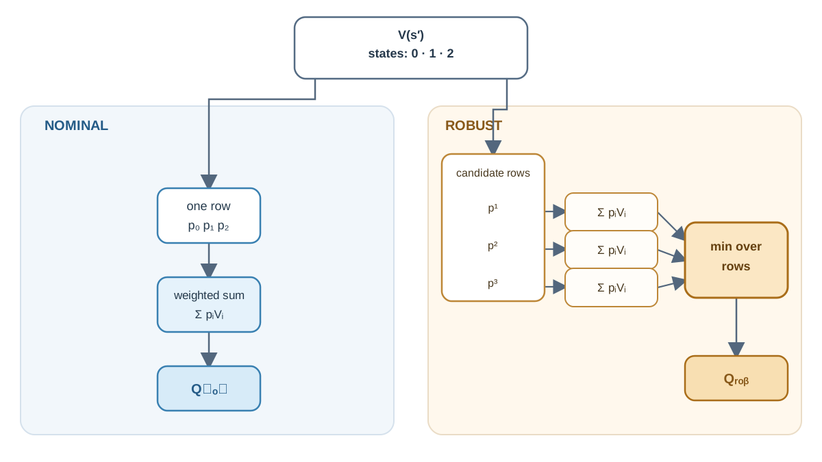
The nominal backup for a state-action pair is:

Q_nominal(s, a) = r(s, a) + gamma * sum over s' of P(s' | s, a) * V(s')

One transition row, one weighted average, done.

The worst-case backup is:

Q_robust(s, a) = r(s, a) + gamma * min over p in P(s, a) of sum over s' of p(s') * V(s')

Read the second line slowly. The minimization is over p, a candidate transition row drawn from the set P(s, a). For each candidate row, you compute the expected next value. Then you keep the smallest result. The min wraps the whole inner sum, not the individual terms.

That distinction is the entire article. If you minimize inside the sum — picking the lowest V(s') and pretending it has probability one — you have answered a different question. You have computed the worst case over next states, not the worst case over models. Those are not the same thing, and the second one is usually far too pessimistic.

Three assumptions keep this experiment clean:

• Rewards are known and identical in both backups. Only the transition row is uncertain.
• The uncertainty set is a set of transition rows. Not a set of value functions, not a set of policies.
• This is planning with a known uncertainty set. It is not a learning algorithm. Nobody is estimating anything from data here.

Common mistake: Treating the uncertainty set as "the set of possible values." It is a set of probability distributions over next states. The value function is a fixed input you supply.

If you want the formal derivation of the robust operator, that ground is covered elsewhere in this curriculum. Here we build the thing and read the output.

The Small MDP and Its Uncertainty Set

We need a problem small enough to verify by hand. Three states, two actions, one genuinely ambiguous transition row.

States are 0, 1, 2. Actions are 0 and 1. Discount factor gamma = 0.9. The value vector we feed into the backup is fixed:

V = [1.0, 5.0, 0.0]

State 1 is the good place to land. State 2 is the bad place. State 0 is mediocre.

Rewards are a plain table, no uncertainty:

R = {
    (0, 0): 1.0, (0, 1): 0.5,
    (1, 0): 0.0, (1, 1): 0.0,
    (2, 0): 2.0, (2, 1): 1.0,
}

Nominal transition rows, written out explicitly so nothing hides in a library:

P_nominal = {
    (0, 0): [0.8, 0.1, 0.1],
    (0, 1): [0.2, 0.7, 0.1],
    (1, 0): [0.1, 0.8, 0.1],
    (1, 1): [0.3, 0.3, 0.4],
    (2, 0): [0.1, 0.1, 0.8],
    (2, 1): [0.4, 0.4, 0.2],
}

Each list is a probability distribution over next states [0, 1, 2].

Now the uncertainty set. We use an L1 ball around the nominal row: every distribution within a stated L1 distance of the nominal row that still sums to one. This is a good teaching choice because the worst case has a closed-form answer, so the code can be checked against arithmetic instead of trusted.

The set is state-action rectangular: nature picks a row for each state-action pair independently. It can adapt to the action, but it cannot coordinate across pairs. That assumption matters, and we will come back to it.

Implementing Both Backups

Plain Python, standard library only. No RL framework, no optimizer.

GAMMA = 0.9
V = [1.0, 5.0, 0.0]

R = {
    (0, 0): 1.0, (0, 1): 0.5,
    (1, 0): 0.0, (1, 1): 0.0,
    (2, 0): 2.0, (2, 1): 1.0,
}

P_nominal = {
    (0, 0): [0.8, 0.1, 0.1],
    (0, 1): [0.2, 0.7, 0.1],
    (1, 0): [0.1, 0.8, 0.1],
    (1, 1): [0.3, 0.3, 0.4],
    (2, 0): [0.1, 0.1, 0.8],
    (2, 1): [0.4, 0.4, 0.2],
}


def nominal_backup(s, a, V):
    row = P_nominal[(s, a)]
    expected = sum(p * v for p, v in zip(row, V))
    return R[(s, a)] + GAMMA * expected


def worst_case_backup(s, a, V, radius):
    """Worst case over an L1 ball of radius `radius` around the nominal row.

    The adversary shifts mass toward the lowest-value next states.
    For an L1 ball, the optimal shift is to move `radius / 2` mass
    from the highest-value state to the lowest-value state, capped
    by the available mass at each end.
    """
    row = P_nominal[(s, a)]
    order = sorted(range(len(V)), key=lambda i: V[i])
    low, high = order[0], order[-1]

    # Total mass the adversary can move is radius / 2.
    shift = min(radius / 2.0, row[high], 1.0 - row[low])

    worst = list(row)
    worst[high] -= shift
    worst[low] += shift

    expected = sum(p * v for p, v in zip(worst, V))
    return R[(s, a)] + GAMMA * expected, worst


def compare(radius):
    print(f"--- radius = {radius} ---")
    print(f"{'state':>5} {'action':>6} {'nominal':>9} {'worst':>9} {'gap':>7}")
    for (s, a) in sorted(P_nominal):
        nom = nominal_backup(s, a, V)
        rob, worst_row = worst_case_backup(s, a, V, radius)
        print(f"{s:>5} {a:>6} {nom:>9.4f} {rob:>9.4f} {nom - rob:>7.4f}")


compare(0.0)
compare(0.4)

The worst_case_backup function does not call a general optimizer. For an L1 ball, the worst case pushes probability mass toward the lowest-value next states, and the amount it can move is bounded by the radius and by how much mass is actually available at the high-value end. Implementing that directly keeps the mechanism visible.

Notice the shape of the function: (s, a, V, radius) in, a scalar out. The backup is a pure function of its inputs. That is deliberate. It means you can change one thing at a time and know exactly what caused the change.

Nominal row: [0.1, 0.8, 0.1]
shift = min(radius / 2.0, row[high], 1.0 - row[low])

Reading the Output

Run the program. With radius = 0.0 you should see:

--- radius = 0.0 ---
state action  nominal     worst     gap
    0      0   2.1700    2.1700  0.0000
    0      1   3.7000    3.7000  0.0000
    1      0   3.7000    3.7000  0.0000
    1      1   3.1500    3.1500  0.0000
    2      0   2.1800    2.1800  0.0000
    2      1   3.4000    3.4000  0.0000

Every gap is zero. This is the first sanity check, and it is not optional. If the radius is zero, the two backups must agree exactly. If they do not, the bug is in your code, not in the theory.

Let's verify one row by hand. State 0, action 0:

r = 1.0
expected = 0.8 * 1.0 + 0.1 * 5.0 + 0.1 * 0.0 = 1.3
Q = 1.0 + 0.9 * 1.3 = 2.17

That matches the printed 2.1700. When the hand arithmetic and the program agree, you have earned the right to trust the rest of the table. When they disagree, one of them is wrong, and you find out which before you build anything on top.

Now raise the radius to 0.4:

--- radius = 0.4 ---
state action  nominal     worst     gap
    0      0   2.1700    1.6300  0.5400
    0      1   3.7000    3.1600  0.5400
    1      0   3.7000    3.4300  0.2700
    1      1   3.1500    2.6100  0.5400
    2      0   2.1800    1.6400  0.5400
    2      1   3.4000    2.8600  0.5400

The gap is the price of the stated uncertainty. It is not an error and it is not noise. It is what you pay for defending against every model in the ball.

Look at state 1, action 0. Its gap is 0.2700, half the others. Why? Its nominal row is [0.1, 0.8, 0.1]. The adversary wants to move mass from state 1 (value 5.0) to state 2 (value 0.0), but it can only move 0.1 out of state 1 before that entry hits zero. The available mass caps the shift. The uncertainty set is not the only constraint — the nominal row is too.

Now check the greedy action under each backup. Nominal: state 0 prefers action 1 (3.70 vs 2.17). Robust: state 0 still prefers action 1 (3.16 vs 1.63). No flip yet. The ranking held.

Warning: If a worst-case value comes out higher than the nominal value, stop. The minimization is being applied to the wrong sign or the wrong object. The worst case over a set that contains the nominal row can never be better than the nominal.

Changing the Uncertainty Set

This is the experiment the article promised. Sweep the radius and watch the robust values fall.

for r in [0.0, 0.2, 0.4, 0.6, 0.8, 1.0]:
    rob_00, _ = worst_case_backup(0, 0, V, r)
    rob_01, _ = worst_case_backup(0, 1, V, r)
    best = 0 if rob_00 > rob_01 else 1
    print(f"radius={r:.1f}  Q(0,0)={rob_00:.4f}  Q(0,1)={rob_01:.4f}  greedy={best}")

As the ball grows, nature can concentrate more mass on the worst next state. The robust value falls. Eventually the fall is uneven — the action whose nominal row had more mass sitting on high-value states has more to lose — and the greedy action flips.

That flip point is the practical signal. It tells you the radius at which your robust policy stops agreeing with your nominal policy. Below it, robustness is cheap insurance. Above it, you are buying protection with performance.

Here is the tradeoff stated plainly: a larger set buys protection against a wider range of models but can select an action that is worse under the true nominal model. Robustness is not free, and the bill is paid in nominal performance.

Common mistake: Building an uncertainty set so large that it includes transition rows that are physically impossible for the environment. That produces meaningless pessimism — you defend against models that cannot occur, and you pay for the privilege.

And the boundary that matters most: a robust policy is not automatically a safe policy. It is optimal only with respect to the set you wrote down. Write a bad set, get a confidently wrong answer.

Where This Breaks Down

The closed-form worst case for an L1 ball does not carry over to general uncertainty sets. Change the set to something without that structure and you need an inner optimization, which is where the real computational cost lives.

State-action rectangularity lets nature adapt per state-action pair. Other rectangularity assumptions — say, letting nature commit to one row per state across all actions — change the answer, sometimes substantially. The set's shape is part of the model, not a detail.

This is a single backup, not value iteration. Repeating robust backups raises separate convergence questions that a one-step calculation cannot answer.

Scaling to many states and actions makes the inner minimization the bottleneck. That is why efficient robust backup algorithms exist and why the research literature spends so much effort on the structure of the set.

What this experiment does not tell you: how to choose the radius from data, and whether the resulting policy transfers to the real environment. Those are separate problems, and they are harder.

Your Next Experiment

Keep the same code and the same printed-table format. Change one thing.

Replace the L1 ball with a per-state interval constraint on each transition probability — a lower and upper bound on p(s') for each next state. The worst case is no longer a single shift; you have to reason about which entries to push to their bounds. Compare the resulting worst-case values to the L1 results.

Or run the robust backup repeatedly to convergence and compare the resulting policy to the nominal value-iteration policy. Or add a second ambiguous state and check whether the action flip happens at the same radius.

The uncertainty set is the real input to a robust backup. So the first question is never "what is the robust value?" It is "what set of models am I actually defending against?" Run the radius sweep. Read the flip point. That number is your answer.