Robust MDPs: Planning With Transition Uncertainty Sets

A planner is only as stable as the model it trusts. Change one transition probability by a few points and watch the preferred action move.

You already know the standard MDP machinery: states, actions, rewards, discounting, and the Bellman relationships that turn a one-step return decomposition into value updates. This article does not re-derive any of that. It changes one assumption. Instead of treating the transition function as a single known object, we treat it as a set of admissible objects and plan against the worst one inside that set.

That single change reshapes the backup operator, and it reshapes the policy. The goal here is to derive the worst-case backup, run it on a small example, and see exactly where the policy's behavior is decided by the shape of the uncertainty set rather than by the reward structure.

Why a Single Transition Model Is a Fragile Assumption

The nominal model is an estimate. Estimation error, model mismatch, and approximation all push the true dynamics away from it. When the estimate is good, planning against it is fine. When it is not, the optimal policy can be sensitive to small probability changes — a nominal optimum is not automatically a stable decision.

It helps to separate two failure sources. The first is uncertainty in the parameters: the true transition probabilities are fixed but unknown, and your estimate is off. The second is uncertainty in the distribution over parameters: the dynamics themselves are drawn from some distribution you only partially know. These are different problems, and they call for different machinery. This article stays with the first, in the finite, tabular, discounted setting.

Note: Robustness is one answer to model error, not the only one. Better data, better features, and shorter planning horizons are alternatives. The question is which response fits the failure you actually have.

Formal Setup: The Robust MDP Tuple and Its Semantics

A robust Markov decision process (RMDP) is a tuple $(S, s_I, A, \mathcal{P}, R, \gamma)$. The states, initial state, actions, reward function, and discount factor are defined as in a standard MDP. What changes is $\mathcal{P}$: instead of a single transition function, it is a set of transition functions, called the uncertainty set or ambiguity set.

Each element $P \in \mathcal{P}$ must still assign a valid probability distribution over next states for every state-action pair. The set constrains which distributions are admissible, but it never lets a single $P$ violate the simplex.

The robust objective is to maximize expected return under the minimizing transition function in the set:

Read this as a game. The agent picks actions to maximize reward. An adversary — nature — picks transitions from $\mathcal{P}$ to minimize it. The policy that survives this game is the robust policy.

There is a semantics question hiding here, and it changes the value of the model. Can the adversary adapt its choice at every step, or must it commit to one transition function for the whole episode? If it can adapt, the worst case is taken per decision. If it must commit, the worst case is taken over whole trajectories. The two produce different values, and the tractable formulation below assumes the adaptive reading.

Rectangularity: The Assumption That Makes Robust Planning Tractable

The structure of the uncertainty set, not just its size, decides whether the problem is solvable.

An s-rectangular set lets the adversary choose transition distributions independently for each state. An s,a-rectangular set extends that independence to each state-action pair. In both cases, the adversary's choices do not interact across the set.

That independence is what makes the worst case decompose per state. If the adversary's choices are independent, the minimum over $\mathcal{P}$ splits into a minimum over each state's admissible distributions, and a local Bellman backup becomes valid. Without it, the choices couple, and the problem becomes substantially harder.

General uncertainty sets make optimal robust policy computation intractable. Tractability is bought with structural assumptions, and rectangularity is the usual price. It is often a modeling convenience rather than a property of the real system — a point worth remembering when you interpret the result.

Deriving the Robust Bellman Backup

Start with the robust value of a fixed policy $\pi$:

Apply the one-step return decomposition. The first reward is fixed by the current state and action; the rest is a discounted continuation:

The reward term does not depend on $P$, so it comes out of the minimization. Under rectangularity, the remaining minimization over $\mathcal{P}$ splits per state, and we get the robust policy-evaluation backup:

The inner minimization is the whole mechanism. Instead of averaging next-state values under the nominal distribution, you assign the worst-case admissible distribution to the next-state values.

For control, add the max over actions outside the inner minimization:

This operator is a two-player, one-step game solved at every state. It remains a contraction under discounting, so value iteration still converges to a fixed point. The derivation assumes finite state and action spaces, a discounted objective, and rectangular uncertainty. Drop any of those and the argument needs repair.

Worked Example: One Small MDP, Two Uncertainty Sets

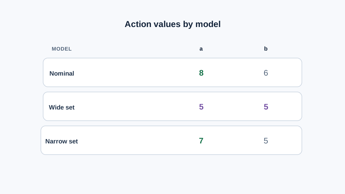
Take three states and two actions. From $s_0$, action $a$ leads to a high-reward state $s_1$ with probability $p$, and to a low-reward state $s_2$ otherwise. Action $b$ leads to $s_1$ with probability $q$. Let $V(s_1) = 10$ and $V(s_2) = 0$, and set $\gamma = 0.9$ so the example stays inside the discounted setting the derivation assumes.

Nominally, $p = 0.8$ and $q = 0.6$. The nominal one-step values from $s_0$ are:

• Action $a$: $0.8 \cdot 10 = 8$
• Action $b$: $0.6 \cdot 10 = 6$

The nominal policy picks $a$.

Now define two uncertainty sets over the same parameters. Both are s,a-rectangular: the adversary chooses $p$ and $q$ independently, so the per-action worst case is well defined and the backup above applies directly.

Set 1 — wide interval: $p \in [0.5, 0.9]$, $q \in [0.5, 0.7]$.

The worst case for action $a$ uses $p = 0.5$, giving $0.5 \cdot 10 = 5$. The worst case for action $b$ uses $q = 0.5$, giving $0.5 \cdot 10 = 5$. The robust values tie, and the policy is no longer decided by the reward structure — it is decided by how wide you drew the interval.

Set 2 — narrow interval: $p \in [0.7, 0.9]$, $q \in [0.5, 0.6]$.

The worst case for action $a$ uses $p = 0.7$, giving $7$. The worst case for action $b$ uses $q = 0.5$, giving $5$. Action $a$ wins again.

Same nominal MDP. Same rewards. Two uncertainty sets, two different robust policies. The flip is not caused by the environment. It is caused by the assumptions you wrote down.

Common mistake: Coupling the parameters — for example, forcing $q = p - 0.2$ — and then minimizing each action independently. That move silently assumes rectangularity. If the real uncertainty couples the parameters, the per-state backup is no longer valid, and the resulting policy may not be robust at all.

Reading the Result: What the Policy Actually Depends On

The robust policy is a function of the uncertainty set, not of the true environment. A wrong set produces a confidently wrong policy, and the confidence is the dangerous part.

Wider sets push toward conservative actions. The cost of that conservatism is the gap between nominal and robust value — in the example above, the robust value of action $a$ drops from 8 to 5 under the wide set. That gap is real return you are choosing not to chase in exchange for protection against a worst case that may never occur.

The adversary's power is bounded by the set. An over-wide set can be more pessimistic than reality warrants, and the resulting policy can underperform the nominal one on the actual system.

Warning: A robust policy is not a safety guarantee. It is optimal against the modeled adversary, not against unmodeled failure. If the real dynamics fall outside your set, the guarantee does not apply.

This connects directly to model-based planning. Robustness is one answer to compounding model error — it bounds the damage from a bad model rather than trying to eliminate the bad model. It is not a replacement for better models.

When Robust Planning Earns Its Cost

Use robust planning when transition estimates are unreliable, when the cost of a bad transition is asymmetric, or when the policy will be deployed outside the data distribution. Stay nominal when the model is well estimated, the environment is stationary, and the conservatism penalty would dominate the risk reduction.

Three failure modes to watch:

1. Treating the uncertainty set as a safety certificate. The set is a modeling choice, not a proof about the world.
2. Assuming rectangularity when the real uncertainty is coupled. If the adversary's choices interact across states, the per-state backup is no longer valid.
3. Scaling the set without checking convergence. The contraction argument holds under discounting and rectangularity. Change those and the value iteration guarantee needs re-examination.

The natural next step is function approximation and partially observable settings, where the same worst-case reasoning reappears with harder computation and the uncertainty set becomes a distribution over beliefs rather than a set of transition matrices.

Where to Take This Next

Return to the opening failure: the policy that flipped when one probability moved. The robust policy is only as meaningful as the uncertainty set you wrote down, and the set is an assumption you own.

Take your own small MDP. Write two candidate uncertainty sets — one wide and independent, one narrow and independent. Run both backups. Compare the resulting policies and the value gaps between them. If the policy flips, you have learned something about your model's fragility. If it does not, you have learned that the decision is stable under your assumptions. Either way, you now know which part of the result came from the environment and which part came from you.