
Deriving the Deterministic Policy Gradient Through the Critic
The deterministic actor loss is one line: maximize $Q(s, \mu_\theta(s))$. It looks like a trick because the log-probability term — the entire engine of the…

Key topics
The deterministic actor loss is one line: maximize . It looks like a trick because the log-probability term — the entire engine of the stochastic policy gradient — has vanished. The gradient did not vanish with it. It moved.
If you already know the likelihood-ratio estimator, you know the shape of the problem. That estimator multiplies a return by , and that log term only exists because is a distribution over actions. A deterministic policy returns one action. There is no density to differentiate, so the estimator collapses to nothing.
The gradient survives anyway, and it comes from a different place: the critic's sensitivity to the action. This article traces that chain link by link — from the objective, through the chain rule, into the update you actually run — and names the assumptions holding it together.
Notation and the Deterministic Objective
Before the derivation, fix the symbols.
- : state.
- : action, assumed continuous.
- : deterministic policy mapping states to actions, parameterized by .
- : action-value function — expected discounted return from taking in and following thereafter.
- : discount factor.
- : state distribution induced by the behavior policy that collects data.
The objective is the expected discounted return of the deterministic policy:
Two things about this expression matter more than they look.
First, the expectation is over states, not state-action pairs. A deterministic policy contributes no action distribution, so there is nothing to average over in action space. The only randomness left is which states you visit.
Second, the state distribution is , not the distribution would induce on its own. This is the off-policy subtlety. Samples come from a behavior policy — typically the deterministic policy plus injected noise, or a separate stochastic explorer — so the states you train on are drawn from someone else's trajectory distribution.
Here is the part that trips people up. depends on in two ways: through the current action , and through the future actions the policy will take after this step. The deterministic policy gradient theorem accounts for both, and its proof carries the future-policy dependence into the state distribution the gradient is taken over. That is why the theorem is stated with an occupancy measure tied to the policy, not an arbitrary behavior distribution.
The practical actor update you write in code does something narrower. It treats the critic as a fixed estimator and differentiates only through the current action, holding the state distribution fixed at whatever the replay buffer provides. That is a semi-gradient: a gradient of a surrogate, not the full theorem-level gradient. It works well enough in practice, and it is what every DDPG-style implementation actually runs — but it is not the same object as the theorem, and conflating them hides the assumption doing the real work.
Knowledge check
Check your understanding
Answer this question before you continue.
The Chain Rule That Carries the Critic Into the Actor
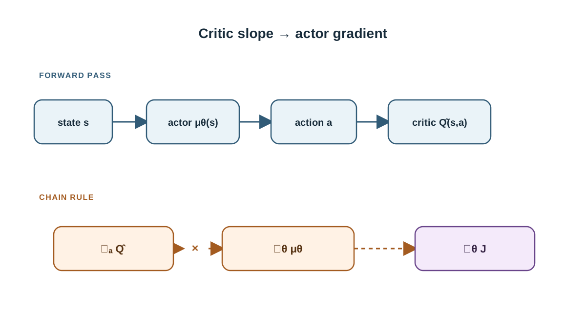
Start from the practical surrogate and differentiate with respect to :
Because is drawn from the replay buffer and treated as a constant with respect to , the gradient passes inside the expectation and touches only the action argument:
Now apply the chain rule. With the critic held fixed, depends on only through the action :
Substituting back gives the actor-through-critic gradient:
Read the two factors as a conversation between two networks.
is the critic answering a question: if I nudge the action in each direction, how does value change? It is a vector in action space, pointing toward higher value.
is the actor answering a different question: if I nudge my parameters, how does my output action move? It is a Jacobian mapping parameter changes to action changes.
Multiply them and you get a vector in parameter space: the direction to move so that the action moves in the direction the critic likes. The critic does not choose the action. It only supplies the slope. The actor supplies the reach.
In practice you estimate this by averaging over a batch of sampled states:
No action sampling. No log-probability. Just a slope and a Jacobian.
Knowledge check
Check your understanding
Answer this question before you continue.
A Worked Example: One State, One Action Dimension
Strip it to the smallest case. One state, one scalar action, one actor parameter.
Suppose the critic near the current action has slope — increasing the action raises value. Suppose the actor's parameter gradient at this state is — increasing raises the output action.
The chain-rule product is:
Gradient ascent on moves the parameter up, which moves the action up, which the critic says is good. The sign is consistent all the way through.
Now flip the critic's slope to . The product is . Gradient ascent moves down, the action drops, and value rises. The actor never needed to know why the critic preferred a smaller action. It only needed the sign and magnitude of the slope.
Geometrically, the actor is being pushed along the direction in which the critic's surface rises fastest, projected through the actor's own parameterization. If the actor cannot express that direction — if is near zero — the critic's slope is multiplied by almost nothing, and the update stalls even when the critic is screaming.
That last observation is the seed of the failure modes.
Knowledge check
Check your understanding
Answer this question before you continue.
What the Derivation Assumes, and What Breaks
The chain-rule product is clean. Reality is not. Each factor carries an assumption, and each assumption has a visible failure mode.
The critic must be differentiable in the action. If is piecewise-constant, uses a non-smooth action path, or is built from operations with zero or undefined gradients in , then is zero or undefined. The actor receives no signal — not a weak signal, no signal. A critic that cannot tell you which way is uphill cannot steer anyone.
The policy must be differentiable in its parameters. Discrete or argmax-style action selection breaks the chain. You cannot differentiate through an . This is why the technique lives in continuous control.
Action bounds and squashing distort the gradient. A or clip applied to the actor output changes the effective . Near the bounds, saturates: its derivative approaches zero, the second factor flattens, and the actor stops responding even when the critic has a strong opinion. If your actions are bounded and your actor keeps pinning them at the limits, suspect saturation before you suspect the critic.
State sampling determines representativeness. The expectation is over . If the behavior policy never visits a region, the actor never receives gradient there. Coverage is not a nicety; it is the sampling assumption made visible.
Critic approximation error becomes actor bias. The actor follows , not . A critic that overestimates value in some action direction will steer the actor in a biased direction, confidently. This is why neighboring algorithms add target critics and delayed updates — the actor is only as good as the slope it is chasing.
Common mistake: Treating a stalled actor as a learning-rate problem. If is near zero because the critic is flat or non-smooth in the action, no learning rate will fix it. Check the critic's action gradient first.
Knowledge check
Check your understanding
Answer this question before you continue.
Deterministic vs Stochastic: Two Different Sources of Gradient
The contrast is the point of the whole derivation.
| Stochastic policy gradient | Deterministic policy gradient | |
|---|---|---|
| Learning signal | Return weighted by | chained through |
| What moves | Probability mass toward actions that paid off | The action itself toward higher value |
| Exploration | From the policy's own distribution | Borrowed from a behavior policy or injected noise |
| Data use | Naturally on-policy | Off-policy estimation from replay, with the target-policy occupancy approximated by behavior states |
| Dominant error | High variance from action sampling | Bias from the critic |
The stochastic gradient shifts a distribution. The deterministic gradient shifts a point. One explores by sampling; the other must import exploration from outside. One is naturally on-policy; the other can reuse a replay buffer because the actor step treats the state distribution as fixed — an approximation, not a free lunch.
The variance-bias trade is the honest summary. The deterministic gradient avoids the high variance of sampling actions, but it inherits whatever bias lives in the critic. You traded a noisy signal for a confident one that might be wrong.
From the Expression to the Update You Actually Run
The practical form is almost embarrassingly short. The actor loss is the negative mean of the critic evaluated at the actor's output:
actor_loss = -critic(states, actor(states)).mean()
actor_loss.backward()
actor_optimizer.step()
Autograd produces exactly the chain-rule product derived above. It computes from the critic, from the actor, and multiplies them on the way back through the graph.
Two implementation details keep the derivation honest.
The state is a constant for the actor step. Only the actor's parameters should receive gradient. The critic's parameters are frozen during the actor update — otherwise you would be changing the slope while you climb it. In code, this is why the critic's parameters are excluded from the actor optimizer, and why some implementations detach the state tensor.
The critic is chasing a moving target. The actor follows the critic's gradient, so an unstable critic produces an unstable actor. Target networks and delayed actor updates exist to slow the critic down enough that the actor is chasing something that holds still for a moment. That machinery is the natural next topic, and it is where the derivation meets engineering.
When not to use this: discrete action spaces, non-differentiable critics, or policies with argmax selection. The chain rule has nothing to grab. Use a likelihood-ratio estimator instead.
The deterministic policy gradient is the critic's action gradient chained through the actor, and it exists only because both the critic and the policy are differentiable in the right places. Everything else — the noise, the replay buffer, the target networks — is scaffolding around that one product.
Your next move: re-derive the chain-rule product on paper for a two-dimensional action, writing out the Jacobian as a matrix and as a row vector. Then open an actor loss in code, set a breakpoint after .backward(), and confirm that the actor's parameter gradients match the two factors you multiplied by hand. When they match, the formula stops being memorized and becomes something you can debug.
Knowledge check
Final check
Finish the article by checking the ideas you just learned.
References
Build a stronger RL mental model
Use structured resources to connect equations, algorithms, and observable agent behavior.


