Deriving Distributional Bellman Updates: Targets, Transforms, and Projection

The scalar Bellman backup hands you a number. The distributional backup has to hand you a shape — and then bend that shape back onto a finite set of atoms.

If you already know how $V$ and $Q$ are derived from the one-step return decomposition, you have the right foundation for this article. What changes here is the object being updated. Instead of tracking a single expected return, we track the entire distribution of returns, and the update rule has to move that distribution correctly through a transition and a reward.

Why the Scalar Target Loses the Information You Need

The ordinary Bellman backup for a policy $\pi$ is:

$Q^\pi(x,a) = \mathbb{E}\big[R(x,a) + \gamma\, Q^\pi(X', A')\big]$

The right-hand side is a single number. It collapses three separate sources of randomness into one expectation: the reward $R$, the next state-action pair $(X', A')$, and the return from that next pair. Once collapsed, you cannot recover the shape of the outcome profile.

Two very different situations can share the same mean. A policy that returns $+1$ every time and a policy that returns $+10$ half the time and $-8$ the other half both have expected return $1$. If your decision depends only on the mean, they are indistinguishable. If your decision depends on variance, tail risk, or multi-modality, they are not.

The distributional view keeps the shape. The price is that the update target is no longer a point — it is a distribution, and it has to be constructed from the next-state distribution through the same transition and reward that the scalar backup uses.

Bridge: This article assumes you have the one-step return decomposition $G_t = R_{t+1} + \gamma G_{t+1}$ and the Bellman expectation and optimality relationships. We will not re-derive those. We will derive what happens when $G$ is treated as a random variable rather than a scalar.

Notation: Return Distributions and the Transition Operator

Let $Z^\pi(x,a)$ be a random variable whose law is the return distribution for state-action pair $(x,a)$ under policy $\pi$. Its expectation is the ordinary action value:

$\mathbb{E}[Z^\pi(x,a)] = Q^\pi(x,a)$

Capital letters mark random variables. Lowercase letters mark realizations. We write $X'$ for the random next state, $A'$ for the random next action, and $R(x,a)$ for the random reward. The standing assumptions are the usual ones: a discounted MDP with discount factor $\gamma \in [0,1)$, bounded rewards, and independence of $R$ and $X'$ given $(x,a)$.

The transition operator $P^\pi$ maps a return-distribution function to the distribution of the next-state return:

$P^\pi Z(x,a) \overset{D}{=} Z(X', A'), \quad X' \sim P(\cdot \mid x,a),\; A' \sim \pi(\cdot \mid X')$

The symbol $\overset{D}{=}$ means equality in distribution. This is the key move: $P^\pi$ does not produce a number. It produces a distribution — the mixture of next-state return distributions weighted by the transition probabilities and the policy.

Deriving the Distributional Bellman Operator

Start from the random-variable recursion:

$Z(x,a) \overset{D}{=} R(x,a) + \gamma\, Z(X', A')$

This is an equality in distribution, not an equality of samples. The left side and the right side are two random variables with the same law. Now substitute the transition operator:

$T^\pi Z(x,a) \overset{D}{=} R(x,a) + \gamma\, P^\pi Z(x,a)$

This is the distributional Bellman operator. Read it as three composed operations on a distribution:

1. Mix. $P^\pi Z(x,a)$ averages the next-state return distributions over all possible $(X', A')$ pairs, weighted by their probabilities.
2. Scale. Multiply by $\gamma$, shrinking the distribution toward zero.
3. Shift. Add $R(x,a)$, translating the distribution along the real line.

The operator is a push-forward: it takes a distribution and pushes it through the affine map $z \mapsto r + \gamma z$. Push-forwards compose linearly, which is why mixing, scaling, and translation combine cleanly into a single operator rather than requiring separate bookkeeping.

Contrast this with the scalar operator. The scalar version collapses randomness at every step. The distributional version propagates it. Same structural shape, fundamentally different object.

For the optimality variant, the greedy action selection replaces the policy expectation. But there is a subtlety: $\max_a \mathbb{E}[Z(x,a)]$ is not the same as a max over distributions. The distributional optimality operator selects the action with the highest expected value, then propagates that action's full distribution. You cannot take a pointwise max of distributions and expect it to correspond to anything meaningful.

Worked Example: One Transition, Three Operations

Consider a two-state MDP. From state $x_1$, action $a$ transitions deterministically to $x_2$ with reward $r = 0.5$. From $x_2$, the policy selects an action whose return distribution is:

$Z(x_2, a') = \begin{cases} 2 & \text{with probability } 0.5 \\ 4 & \text{with probability } 0.5 \end{cases}$

Let $\gamma = 0.9$. We compute the target distribution $T^\pi Z(x_1, a)$ step by step.

Step 1: Mix. Since the transition is deterministic, $P^\pi Z(x_1, a) = Z(x_2, a')$. The distribution is unchanged: atoms at 2 and 4, each with probability 0.5.

Step 2: Scale. Multiply each atom by $\gamma = 0.9$: atoms at $1.8$ and $3.6$, each with probability 0.5.

Step 3: Shift. Add $r = 0.5$: atoms at $2.3$ and $4.1$, each with probability 0.5.

The target distribution has support $\{2.3, 4.1\}$ with equal probability. Its mean is $3.2$. The scalar backup gives $0.5 + 0.9 \times 3 = 3.2$. The means agree — as they must, since expectation is linear and the distributional operator is a strict refinement.

Geometrically: discounting is a contraction toward the origin, the reward is a translation, and the mixture is a weighted average of shapes. If the transition were stochastic, step 1 would produce a mixture of two or more distributions before scaling and shifting.

Why the Target Usually Lands Off the Support

A categorical representation fixes a finite set of atoms $z_0, z_1, \ldots, z_{N-1}$, typically evenly spaced on $[V_{\min}, V_{\max}]$. The transformed target $r + \gamma z_j$ generally falls between atoms. In the example above, if the support were $\{0, 1, 2, 3, 4, 5\}$, the target atoms at $2.3$ and $4.1$ do not coincide with any grid point.

The target is therefore a distribution the current parameterization cannot represent exactly. This is not a numerical precision issue. It is a representational mismatch — the same problem as fitting a continuous density with a discrete histogram. The histogram can approximate the density, but it cannot equal it.

Common mistake: Skipping projection and regressing directly on the raw transformed atoms. This silently biases the learned distribution because the network is being asked to place probability mass at locations its output layer cannot express. The loss may decrease, but the distribution drifts.

Projection: Bending the Target Back Onto the Support

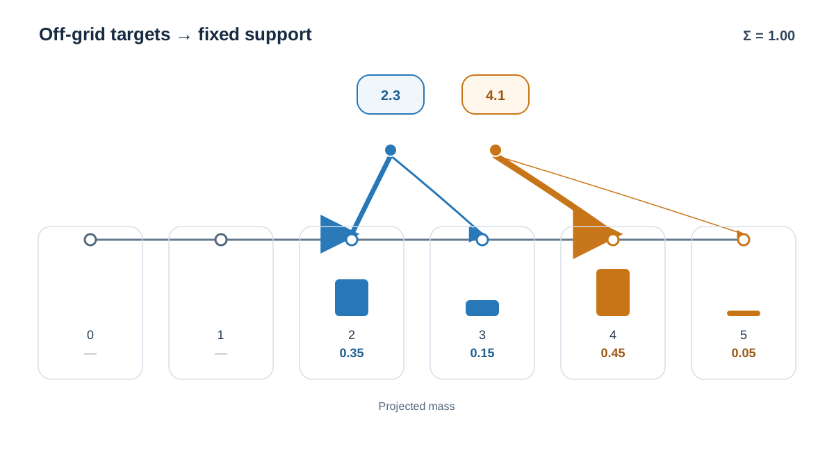
Projection $\Phi$ maps an arbitrary distribution onto the fixed support by distributing each atom's probability to its immediate neighbors, weighted by inverse distance. If a transformed atom $\hat{z}_j = r + \gamma z_j$ falls between $z_i$ and $z_{i+1}$, its probability $p_j$ is split:

$(\Phi \hat{Z})_i \mathrel{+}= \left(1 - \frac{|\hat{z}_j - z_i|}{\Delta z}\right) p_j, \quad (\Phi \hat{Z})_{i+1} \mathrel{+}= \left(1 - \frac{|z_{i+1} - \hat{z}_j|}{\Delta z}\right) p_j$

where $\Delta z = z_{i+1} - z_i$. The allocation is piecewise linear and mass-preserving: total probability is conserved, but the support is not. The projected distribution lives on the original grid.

Let's continue the example. Suppose the support is $\{0, 1, 2, 3, 4, 5\}$, so $\Delta z = 1$. The first target atom is $\hat{z}_1 = 2.3$. It falls between $z_2 = 2$ and $z_3 = 3$. Its probability $p_1 = 0.5$ splits as:

• To $z_2 = 2$: $(1 - |2.3 - 2|/1) \times 0.5 = 0.7 \times 0.5 = 0.35$
• To $z_3 = 3$: $(1 - |3 - 2.3|/1) \times 0.5 = 0.3 \times 0.5 = 0.15$

The second target atom is $\hat{z}_2 = 4.1$. It falls between $z_4 = 4$ and $z_5 = 5$. Its probability $p_2 = 0.5$ splits as:

• To $z_4 = 4$: $(1 - |4.1 - 4|/1) \times 0.5 = 0.9 \times 0.5 = 0.45$
• To $z_5 = 5$: $(1 - |5 - 4.1|/1) \times 0.5 = 0.1 \times 0.5 = 0.05$

The projected distribution on the grid is:

Atom	Probability
0	0.00
1	0.00
2	0.35
3	0.15
4	0.45
5	0.05

Check the mass: $0.35 + 0.15 + 0.45 + 0.05 = 1.0$. Check the mean: $0 \times 0 + 1 \times 0 + 2 \times 0.35 + 3 \times 0.15 + 4 \times 0.45 + 5 \times 0.05 = 0.7 + 0.45 + 1.8 + 0.25 = 3.2$. The projected mean matches the unprojected mean exactly. That is not a coincidence — piecewise linear interpolation preserves the first moment when the target atoms fall inside the support. It does not preserve higher moments, and it does not preserve the mean when mass is clipped at the boundaries.

The projected operator $\Phi T^\pi$ is a contraction in an appropriate metric (the Cramér distance, for the categorical case), so the fixed-point reasoning from the scalar case carries over with a caveat: the fixed point is now a fixed point of the projected operator, not of the original one.

What projection loses: fine structure between atoms, and exactness when the target's support lies far outside $[V_{\min}, V_{\max}]$. Boundary behavior matters. Mass pushed past the support edges is clipped onto the nearest atom, which is a real source of bias in practice. If your returns routinely exceed $V_{\max}$, the learned distribution will pile probability at the boundary and understate tail risk.

From Projected Target to Update Rule

The update minimizes a divergence between the projected target distribution and the current predicted distribution. In the categorical case, this is a cross-entropy term:

$L(\theta) = -\sum_i (\Phi \hat{Z})_i \log Z_\theta(x,a)_i$

This turns the Bellman update into a classification problem over atoms. That is why the loss looks like multiclass cross-entropy rather than squared error. The next-state distribution is treated as fixed — parameterized by a target network or a frozen copy of $\theta$ — so the update is a stable regression toward a moving target.

Contrast with the scalar case: squared error on a point estimate versus a distributional divergence on a histogram. The scalar update asks "how far is my number from the target number?" The distributional update asks "how far is my histogram from the projected target histogram?"

What the Distributional View Changes, and What It Does Not

The expectation of the learned distribution still recovers the ordinary value. The distributional view is a strict refinement, not a replacement. It earns its cost when outcome variability is decision-relevant: risk-sensitive control, multi-modal returns, or diagnosing why a policy is unstable despite a reasonable mean.

But here is the boundary that trips people up: predicting a return distribution does not, by itself, make the policy risk-sensitive. The standard expectation-greedy update described in this article still selects actions by the highest mean. If you want to act on the tail, the variance, or a specific quantile, you need an additional decision rule that reads the distribution and chooses accordingly. The distribution is information; the risk criterion is a separate choice about how to use that information. Conflating the two leads to the mistaken belief that switching from DQN to C51 automatically produces risk-aware behavior. It does not.

It also does not fix exploration, credit assignment, or function-approximation instability. Those are separate problems. And the clean contraction story assumes a fixed support and a tabular or well-behaved parameterization. Deep function approximation reintroduces the usual convergence caveats.

The cost is real: more parameters, a projection step per update, and sensitivity to support bounds and atom count. If you only need the expected return, keep the scalar backup. If the shape of the return changes your decision, carry the distribution and accept projection as the price of a finite representation.

Next Step

Build the three operations by hand. Take the two-state example above, write a short script that represents $Z(x_2, a')$ as a list of atoms and probabilities, applies mix, scale, and shift, then projects onto a fixed grid. Verify that the projected target's mean matches the scalar backup. Then push one target atom past $V_{\max}$ and watch the mean drift — that is the boundary bias in action, and it is the failure mode most worth internalizing before you tune a real agent. When the numbers agree, you have confirmed the derivation against output rather than trusting it. When they disagree, you have found either a projection bug or a boundary case worth understanding.