
How Model Error Propagates Across a Finite Planning Horizon
A planner that looks accurate one step ahead can still produce value estimates that drift badly over a rollout. The usual reaction is to blame the model.…

Key topics
A planner that looks accurate one step ahead can still produce value estimates that drift badly over a rollout. The usual reaction is to blame the model. The more useful reaction is to ask a sharper question: how much error does one step contribute, and how does the horizon spend it?
This is the quantitative version of the compounding-error intuition. Here we make the bound explicit, separate the reward-model contribution from the transition-model contribution, and turn the result into a rule for choosing a planning horizon.
What You Are Actually Bounding
Fix a policy . You have two models of the same environment: the true transition and reward model , and a learned approximation . Under each model you can roll out the policy for steps and compute a finite-horizon value.
The object of study is the gap between those two values:
where is the value predicted by planning under the learned model and is the value under the true model, both for the same fixed policy and the same starting state .
Two things are worth stating before any algebra.
First, this is a value-prediction error, not a policy-performance error. The bound tells you how wrong your value estimate is for a policy you already have. It says nothing about how good the policy you extract from that estimate will be. That distinction matters later, because it is the most common place readers over-claim the result.
Second, the bound is conditional. It holds under explicit assumptions about bounded rewards, a bounded per-step model error, and a value function that does not change too violently when the next-state distribution shifts. If those assumptions fail, the bound fails with them.
The intuition article in this series established that model error compounds across imagined rollouts. The bound is what makes that compounding predictable instead of anecdotal.
Notation and Assumptions Before Any Derivation
Define everything before using it.
| Symbol | Meaning |
|---|---|
| state and action | |
| fixed policy being evaluated | |
| discount factor | |
| planning horizon (number of imagined steps) | |
| true transition distribution | |
| learned transition distribution | |
| true expected reward | |
| learned expected reward | |
| bound on $ | |
| per-step reward-model error bound | |
| per-step transition distance between and | |
| Lipschitz constant of the value function |
The assumptions, stated plainly:
- Bounded rewards. and for all .
- Bounded reward error. for all .
- Bounded transition error. for all , where is a distance between probability distributions.
- Lipschitz value. For any two next-state distributions , the induced expected continuation values differ by at most .
Why measure transition error as a distance between distributions rather than a difference in parameters? Because the value function only sees the distribution. Two parameterizations can differ wildly while producing nearly identical distributions, and two nearly identical parameterizations can produce very different distributions. The distance that matters is the one the value function can feel.
The Lipschitz assumption is the load-bearing one. It says a small shift in the next-state distribution produces a bounded shift in expected value. When the value function is nearly flat in some region, is small and transition error barely matters. When value changes sharply across neighboring states, is large and even a tiny distribution shift can move the value estimate a lot.
What breaks when these assumptions fail: unbounded rewards make meaningless, a non-Lipschitz value function makes the transition term unbounded, and a horizon that exceeds the discount's effective reach makes the geometric sum saturate rather than grow.
Deriving the One-Step Error
Start with the one-step Bellman-style value under each model, for a fixed policy:
Subtract and take absolute values. The expectation over actions is linear, so it passes through:
The first term is the reward contribution. By assumption 2, it is bounded by .
The second term is the transition contribution. The inner difference is exactly the kind of quantity the Lipschitz assumption controls: a change in the next-state distribution produces a change in expected value bounded by times the distribution distance. So:
Putting it together, the one-step error bound is:
Read that carefully. One step of planning error has two independent sources, and they do not cancel. A perfect transition model does not save you from a bad reward model, and a perfect reward model does not save you from a bad transition model. If you are debugging a drifting planner, this is the first place to look: which term is larger?
Knowledge check
Check your understanding
Answer this question before you continue.
Compounding Across H Steps
Now extend to steps by induction. The key requirement is that the Lipschitz constant must bound the distribution-sensitivity of every continuation value used through horizon , not just the one-step value . If the value function's Lipschitz constant varies with the remaining horizon, use the maximum over all horizons up to . Call that uniform bound .
Let denote the error at horizon , with since both models agree on the terminal value.
At horizon , the error decomposes into the one-step reward error plus the discounted transition error applied to the continuation value at horizon :
This recurrence is the engine of the whole result. Each new step adds a fixed per-step error , then discounts the accumulated error from all previous steps by . The transition contribution appears at every depth because the Lipschitz condition holds uniformly across all continuation values.
Unrolling the recurrence from :
Using the closed form for a finite geometric series:
So the bound becomes:
This is the finite-horizon model error bound. Two features matter.
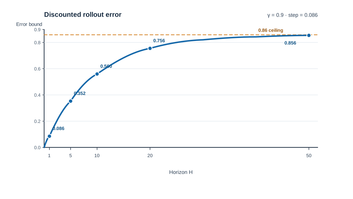
The factor grows with but saturates. As , it approaches 1, and the whole bound approaches . That ceiling is the discount-limited maximum error. You cannot accumulate more than that, no matter how long you plan.
The horizon still matters, but only in the regime where is not yet negligible. When per-step error is large, the ceiling is high and you hit it fast. When per-step error is small, the ceiling is low and the horizon barely changes the answer.
Note: The bound is an upper bound under the stated assumptions. Real error is often smaller, sometimes much smaller. Treat it as a worst-case envelope, not a prediction.
Knowledge check
Check your understanding
Answer this question before you continue.
A Worked Numeric Example
Pick small numbers so the arithmetic stays visible. Let , , , and .
The per-step transition contribution is . The reward contribution is . Reward error dominates here, roughly 58% of the one-step total.
The ceiling is .
Now compute the bound at three horizons:
| Bound | ||
|---|---|---|
| 1 | 0.10 | 0.086 |
| 5 | 0.41 | 0.353 |
| 10 | 0.65 | 0.559 |
| 20 | 0.88 | 0.757 |
| 50 | 0.995 | 0.856 |
The bound climbs steeply for the first ten steps, then flattens. By you are within 1% of the ceiling. Increasing the horizon past roughly 20 buys almost nothing in accuracy terms, which means the extra computation is pure cost.
Now flip the case. Suppose instead of , so the transition contribution is and the reward contribution stays at . Transition error now dominates, roughly 88% of the one-step total. The ceiling jumps to .
The practical implication is direct. In the first case, spend your modeling effort on the reward model. In the second, spend it on the transition model. The bound tells you where the leverage is.
Knowledge check
Check your understanding
Answer this question before you continue.
Reading the Bound as a Replanning Rule
The bound is not just a diagnostic. It is a decision rule.
Shortening the horizon reduces accumulated error but also reduces foresight. The bound quantifies the accuracy cost of that trade. If you cut from 20 to 5 in the first example, you drop the worst-case error from 0.757 to 0.353, but you also lose 15 steps of lookahead. Whether that trade is worth it depends on how much the later steps would have changed your action.
Replanning limits the depth of each imagined rollout. When you replan from a fresh real observation, the next prediction starts from a state you actually observed rather than from a model-generated state. This caps the open-loop rollout depth at the segment length between real observations. The bound applies per segment, not across the whole episode. But be careful about what this does and does not guarantee: replanning restarts the prediction from real data, yet this fixed-policy bound alone does not establish that errors across repeated replans cannot affect episode-level performance or the quality of the policy you extract. The bound describes value prediction for a fixed policy, and replanning generally changes the policy and the sequence of decisions.
State-dependent horizons make sense. If is large in some states and small in others, the bound is larger in those states. A state where the model is untrustworthy deserves a shorter horizon than a state where the model is accurate. This is the principle behind adaptive-horizon methods that choose per state based on estimated cumulative model error.
When the bound is too loose to be useful. If per-step error is large and the effective horizon is long, the ceiling is high enough that the model should not be trusted for planning at all. At that point, model-free updates or a much shorter horizon with heavy replanning are the honest options.
Knowledge check
Check your understanding
Answer this question before you continue.
Common Mistakes When Applying This Bound
Treating the bound as tight. It is an upper bound under assumptions. Real error is often smaller. Do not use it to predict exact error; use it to compare contributions and set a ceiling.
Ignoring the Lipschitz constant. A large can make the transition term dominate even when looks small. If value changes sharply across neighboring states, transition error is amplified. Measure or estimate before concluding that transition error is negligible.
Assuming the bound covers policy improvement. It bounds value prediction for a fixed policy. The policy you extract from that value estimate is a separate question, and the bound does not answer it.
Forgetting that the bound assumes the same policy under both models. In practice, the policy you evaluate under the learned model may differ from the policy the true model would induce. That gap is not covered here.
Common mistake: Concluding that a small means transition error does not matter. Multiply by and first. The product is what enters the bound.
What This Bound Does Not Tell You
The bound is a tool with a specific shape. Knowing its edges keeps you from over-claiming.
It does not bound policy performance after improvement. It bounds value prediction under a fixed policy. If you use the predicted value to pick a better policy, the quality of that policy is a separate analysis.
It does not handle function approximation error. If your value function is itself an approximation, that adds a separate term, often larger than the model error term. The bound here assumes you can evaluate the value function exactly.
It does not tell you the true model error. It tells you what happens given a per-step error you must estimate separately. The bound is only as useful as your estimate of and .
The concrete next step is to estimate per-step model error empirically. Hold out real transitions, compare predicted next-state distributions to observed ones, and compute a distribution distance. Do the same for rewards. Plug those numbers into the geometric bound, and let the resulting accuracy ceiling choose your horizon instead of picking one by feel.
That is the whole point of the bound. It turns "the model is wrong" into "the model is wrong by this much per step, and here is what the horizon does with it."
Knowledge check
Final check
Finish the article by checking the ideas you just learned.
References
Build a stronger RL mental model
Use structured resources to connect equations, algorithms, and observable agent behavior.


