
When Does Tabular Q-Learning Converge? Conditions and Limits
Your Q-table went quiet. The values stopped moving, the greedy policy stopped changing, and the learning curve flattened into something that looks like a…

Key topics
Your Q-table went quiet. The values stopped moving, the greedy policy stopped changing, and the learning curve flattened into something that looks like a settled answer. It is tempting to call that convergence. But a table going quiet is an observation. Convergence is a theorem with preconditions, and the theorem does not care how calm your plot looks.
Here is the reframe that matters: the Q-learning update supplies the direction of travel, and the way you generate experience plus the way you shrink your step size supply the guarantee. Change either of those and you are no longer covered by the classical result, no matter how correct the update line looks.
What the Convergence Claim Actually Says
Before testing anything, pin down the exact promise. The classical result for tabular Q-learning says that as the number of updates goes to infinity, the estimate approaches the optimal action-value function with probability 1.
Three words in that sentence do most of the work.
Asymptotic. The claim is about a limit, not about episode 500 or step 50,000. There is no "converges after N episodes" clause. Any finite snapshot, including the one where your table looks stable, is compatible with both convergence and slow drift.
Tabular. The claim lives in a finite MDP: a finite state set, a finite action set, and one independent entry per state-action pair. That independence is not a detail. It is load-bearing, and it is the first thing to disappear when you replace the table with a function.
Discounted. The discount factor is strictly below 1, which keeps returns finite and gives the iteration a fixed point to aim at.
To fix notation, let be a state, an action, the reward received, the discount factor, and the step size applied to pair at update . If counts how many times that pair has been updated so far, the update is:
You have seen this before, so treat it as a notation anchor rather than a lesson. The bracket is the observed bootstrapped target minus the current estimate. When it is positive, the update pushes upward; when it is negative, it pulls the estimate down. The step size decides how much of that gap you absorb.
Notice what the update does not contain. It says nothing about which pairs you visit, how often, or whether your step size shrinks. Those decisions live outside the equation, and they are exactly where the convergence conditions live.
Knowledge check
Check your understanding
Answer this question before you continue.
The Two Conditions That Do the Work
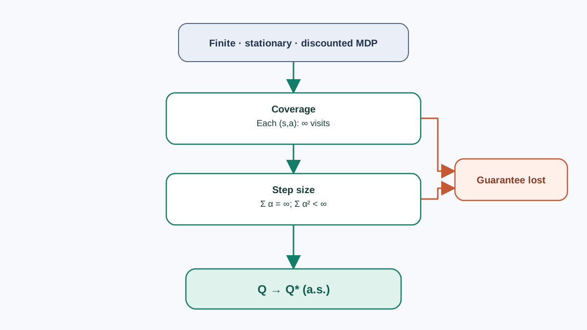
The theorem reduces to two requirements. They are usually recited as ritual. They are more useful as mechanisms.
Condition one: every state-action pair must be visited infinitely often. Not frequently. Not on average. Infinitely often, with probability 1. The theorem does not care which exploration policy produces this coverage, only that no pair is permanently starved of evidence.
Condition two: the step sizes must satisfy the Robbins-Monro schedule. For each pair, the sum of step sizes over its visits must diverge, while the sum of their squares must converge:
Why this particular pair of conditions, and not some other? Because each one guards a different failure.
The divergent sum guarantees the estimate can still travel. If your initial values are badly wrong, a step size that shrinks too fast locks in the error before the updates have had room to correct it. The sum being infinite means there is always enough total movement budget left to reach the truth.
The convergent square sum guarantees the noise dies. Every update injects sampling noise from a single observed reward and a single next state. If the squares keep summing to something finite, the cumulative variance of those injections stays bounded, and the estimate can settle instead of jittering forever.
The two conditions pull in opposite directions on purpose. One keeps the door open; the other closes it gradually. A schedule like satisfies both. A constant step size satisfies the first and violates the second.
Common mistake: Treating a constant learning rate as a bug. It is not. A constant step size is a deliberate engineering choice that buys responsiveness and tracking in non-stationary settings. What it does not buy is the classical convergence guarantee. You get a bounded oscillation band instead of a settled value, and that band is the price, not a defect.
The visitation condition deserves the same scrutiny. It is a statement about coverage, not about cleverness. An -greedy policy with a fixed, non-zero keeps every action reachable from every state you actually visit, but reachability is not the same as visitation. If the environment's transition structure makes some states unreachable from your start distribution, no amount of action randomness will visit the pairs inside them. And even when every pair is reachable, the theorem's condition is about the infinite limit: you need evidence that coverage persists, not a finite count that happens to look healthy.
A policy that locks onto a good action early and stops exploring fails the condition outright, even if it performs beautifully. Coverage is the requirement; optimism, curiosity, and reward shaping are optional extras that may or may not help you get there.
Knowledge check
Check your understanding
Answer this question before you continue.
A Worked Trace: Watching the Conditions Bite
Abstract conditions become believable when you watch them fail. Take a three-state chain: , two actions per state, a reward of on the transition into and elsewhere, and . The optimal values are small enough to check by hand, which is the point: you want a target you can verify without trusting the algorithm.
Start with one concrete update. Suppose the agent is in , takes action , receives reward , and lands in . The current estimates are and . The bootstrapped target is:
The gap between target and current estimate is . If this is the first update to , then , and the new estimate becomes . On the second visit, , and the same gap would move the estimate only halfway. That shrinking step size is the Robbins-Monro schedule doing its job: large corrections early, gentle refinements later.
Now run three variants and compare.
| Variant | Step size | Visitation | What you observe |
|---|---|---|---|
| A | -greedy, fixed | Estimates settle toward the hand-computed values | |
| B | constant | -greedy, fixed | Estimates oscillate inside a stable band |
| C | greedy after 300 steps | Most pairs converge; one pair freezes wrong |
Variant A is the textbook case. Both conditions hold, and the values walk toward the target and stay there.
Variant B is the one that trips people up. The estimates do not diverge. They wobble around the right neighborhood and never fully commit. That wobble is not a bug in your code and not a sign that Q-learning "failed." It is the second condition being violated on purpose, and the bounded band is exactly what you should expect.
Variant C is the instructive failure. Suppose the pair is only ever tried during the first few hundred steps, before the policy turns greedy. Its estimate freezes at whatever value it held when the visits stopped. Every other pair converges cleanly, which makes the frozen entry easy to miss. That entry is not learning slowly. It is learning nothing, because the evidence stopped arriving. The coverage clause is not decoration; it is the difference between a wrong number and a right one.
You can verify the mechanism with a short snippet rather than a full implementation. Track two arrays alongside your Q-table: visit counts per pair, and the step size used on the last update to each pair.
visits = {}      # (s, a) -> count
last_alpha = {}  # (s, a) -> step size used

def update(q, s, a, r, s_next, gamma):
    n = visits.get((s, a), 0) + 1
    visits[(s, a)] = n
    alpha = 1.0 / n          # satisfies both Robbins-Monro sums
    last_alpha[(s, a)] = alpha
    td_error = r + gamma * max(q[s_next].values()) - q[s][a]
    q[s][a] += alpha * td_error
After training, sort visits ascending. The pairs at the bottom of that list are your convergence suspects, and they will explain more failed runs than any hyperparameter sweep.
Knowledge check
Check your understanding
Answer this question before you continue.
Why the Discount Factor and the MDP Assumptions Matter
The two headline conditions get the attention. The quieter assumptions do the structural work, and each one is cheap in a textbook MDP and expensive in a real one.
The discount factor stays strictly below 1. This keeps returns finite and makes the Bellman operator a contraction, which is what gives the iteration something to converge toward. At in a continuing task, returns can grow without bound and the contraction argument loses its footing.
The environment is stationary. Rewards and transitions do not change underneath the learner. If they do, you are no longer asking a convergence question. You are asking a tracking question, and the answer is different: a constant step size becomes the right tool precisely because the target is moving.
The tabular representation keeps entries independent. An update to one pair cannot corrupt another, because each pair owns its own number. This is the assumption that quietly disappears the moment a neural network replaces the table, and it is the one most people never notice they were relying on.
Rewards are bounded. The contraction argument needs a finite scale to work against. Unbounded rewards break it even though the update line looks unchanged.
Note: These are the fine print of the theorem. Satisfying them in a gridworld takes one line of setup. Satisfying them in a production system with drifting user behavior, delayed rewards, and a learned state encoder is a research program, not a configuration flag.
Knowledge check
Check your understanding
Answer this question before you continue.
Where the Guarantee Stops
Everything above is a statement about a table with one independent entry per pair. Replace the table with a parameterized function and the independence assumption is gone. An update to changes the estimate for every pair, including pairs you have not visited recently.
That single change breaks the argument in a specific way. With function approximation, the update is no longer a contraction in the same space, and the fixed point of the update can differ from the fixed point of the Bellman equation. Divergence is possible, not hypothetical. The combination of function approximation, bootstrapping, and off-policy data is the configuration that makes it likely, and it is exactly the configuration deep Q-learning uses.
This is why a deep Q-learning convergence guarantee is a separate research problem with its own conditions, not a corollary you inherit from the tabular result. The tabular theorem is a proof. The deep result is a set of conditions under which behavior is usually stable in practice, supported by engineering choices: target networks that freeze the bootstrap target, replay buffers that decorrelate samples, gradient clipping, and conservative step sizes. Those choices are not the theorem. They are substitutes for it.
Warning: Do not carry the tabular guarantee into a deep setting by habit. "Q-learning converges" is true under stated conditions in the tabular case and unproven in the general function-approximation case. Confusing the two turns a precise result into a false sense of safety.
A Practical Checklist Before You Trust a Converged Table
Theory is only useful if it changes what you check. Run this against your own experiment before you conclude anything.
Check coverage first. Count visits per state-action pair. If some pairs have a handful of updates, you have a coverage problem, not an algorithm problem. Fix the exploration before you touch the learning rate. Remember that a finite count is evidence, not proof: the theorem's condition is about persistent visitation in the limit, so you are looking for signs that coverage continues, not a threshold that certifies it.
Check the step size. If it is constant, expect a bounded oscillation band and stop reading that band as failure. If it decays, confirm it decays slowly enough that the sum still diverges.
Check the environment. If rewards or transitions changed during training, the target moved and your estimate is chasing it. That is tracking, and it is a different claim.
Check the scale. A table that looks converged on a small MDP tells you nothing about whether the same update will behave under function approximation. The result does not transfer by default.
The decision rule is short: trust the convergence claim only when coverage is persistent, the step size decays, and the environment is stationary. Otherwise you are observing stability, and stability is not the same thing as convergence.
Where to Go Next
Instrument your own tabular experiment. Log visit counts and step sizes per pair, then deliberately break one condition at a time. Switch to a constant step size and watch the oscillation band appear. Cut exploration early and find the frozen entry. Each failure mode maps to a specific clause in the theorem, and seeing them in your own output is worth more than reading the conditions twice.
Once you can predict which failure you will get before you run it, you are ready for the boundary itself: what happens when the table becomes a network, and why the guarantee you just learned stops applying there.
Knowledge check
Final check
Finish the article by checking the ideas you just learned.
References
Build a stronger RL mental model
Use structured resources to connect equations, algorithms, and observable agent behavior.


